Eigenvalue Classification of Symmetric Matrices

Hello! Welcome back to our study of symmetric operators.

In the last lesson, we introduced the concepts of positive definite and positive semi-definite matrices. We defined them based on the sign of the quadratic form, $x^{T} A x$ , which we interpreted as the "energy" of a system or the geometric relationship between an input vector $x$ and its transformation $A x$ . We noted that while this definition is fundamental, testing it for all possible vectors is impossible.

Today, we'll build on that foundation by connecting definiteness to a much more practical tool: eigenvalues. Our learning outcome is to classify a symmetric matrix as positive definite, semi-definite, or indefinite using its eigenvalues. As we've seen, the Spectral Theorem guarantees that a symmetric matrix's eigenvalues are always real, making this a reliable and powerful method.

1. The Eigenvalue Test for Definiteness

The most important takeaway from this lesson will be a set of simple rules that link the signs of a symmetric matrix's eigenvalues to its definiteness classification. This is the practical payoff from our study of the Spectral Theorem.

The following resources provide a clear and direct statement of these rules.

Definite matrix

The 'Eigenvalues' section of this Wikipedia article provides the definitive rules connecting eigenvalues to definiteness. This is the core of today's lesson.

Read the short section titled 'Eigenvalues'. Focus on the five bullet points that state the 'if and only if' conditions for each classification.

2.7: Critical Points

These notes from the University of Toronto offer a slightly different presentation of the same theorem and also explicitly state the rules for negative definite/semidefinite cases.

Read the subsection 'Eigenvalues of definite matrices', down to just before 'Example 1'. This section clearly lays out the theorem and its implications.

Let's summarize these crucial rules for an $n \times n$ symmetric matrix $A$ with eigenvalues $λ_{1}, \dots, λ_{n}$ :

Classification	Condition on Eigenvalues $λ_{i}$
Positive Definite	All $λ_{i} > 0$
Positive Semi-definite	All $λ_{i} \geq 0$ (with at least one $= 0$ )
Negative Definite	All $λ_{i} < 0$
Negative Semi-definite	All $λ_{i} \leq 0$ (with at least one $= 0$ )
Indefinite	Has both positive ( $λ_{i} > 0$ ) and negative ( $λ_{j} < 0$ ) eigenvalues.

Why does this work? Recall from our previous lesson that a matrix is positive definite if $x^{T} A x > 0$ . If $v$ is an eigenvector with eigenvalue $λ$ , then:
$v^{T} A v = v^{T} (λ v) = λ (v^{T} v) = λ ∥ v ∥^{2}$
Since $∥ v ∥^{2}$ is always positive, the sign of $v^{T} A v$ is determined entirely by the sign of $λ$ . Because the eigenvectors of a symmetric matrix form a complete basis for the space, this relationship extends to any vector $x$ , not just eigenvectors.

The following video gives a great visual explanation of this connection.

What Does It Mean For a Matrix to be POSITIVE? The Practical Guide to Semidefinite Programming(1/4)

This video from 'Visually Explained' provides an excellent intuition for why the eigenvalue signs determine the definiteness of the matrix.

Watch from 6:02 to 7:34. The animation clearly shows how a positive eigenvalue scales an eigenvector, while a negative eigenvalue reflects and scales it, violating the 'same side' condition required for positive definiteness.

Test your understanding!

Consider the matrix $A = 300 0 - 2 0 001$ . Since it's a diagonal matrix, its eigenvalues are simply its diagonal entries. How would you classify this matrix?

Show answer

The eigenvalues are $λ_{1} = 3$ , $λ_{2} = - 2$ , and $λ_{3} = 1$ . Since the matrix has both positive and negative eigenvalues, it is indefinite.

2. Visualizing Definiteness through Quadratic Forms

The signs of the eigenvalues directly determine the shape of the surface defined by the quadratic form $f (x) = x^{T} A x$ . Given your background in multivariable calculus, you can visualize these as surfaces in 3D for a $2 \times 2$ matrix.

Visualizing Quadratic Forms and Matrix Definiteness — This figure illustrates the connection between matrix definiteness and the geometry of the corresponding quadratic form $f(x_1, x_2) = \mathbf{x}^T A \mathbf{x}$. A positive definite matrix corresponds to a 'bowl' shape (minimum). A negative definite matrix corresponds to an inverted 'bowl' (maximum). A positive semi-definite matrix forms a 'trough' with a line of minima. An indefinite matrix forms a 'saddle' point.

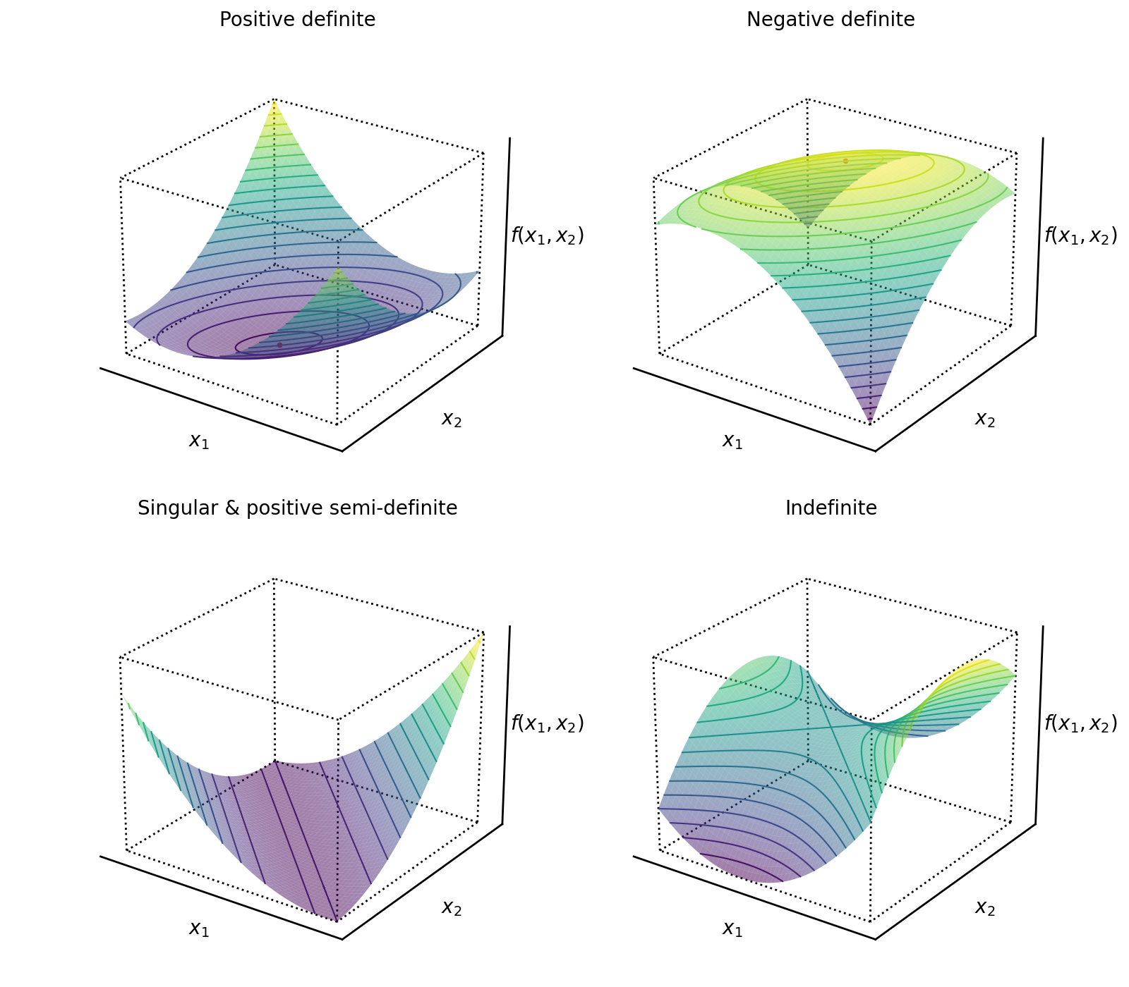
Let's connect these shapes to our eigenvalue rules:

Positive Definite (all $λ_{i} > 0$ ): The surface is a paraboloid opening upwards, with a unique global minimum at the origin. Think of the function $f (x, y) = x^{2} + y^{2}$ .
Negative Definite (all $λ_{i} < 0$ ): The surface is an inverted paraboloid opening downwards, with a unique global maximum at the origin. Think of $f (x, y) = - x^{2} - y^{2}$ .
Positive Semi-definite (all $λ_{i} \geq 0$ , one is 0): The surface is a parabolic "trough" or "valley". It has a minimum value of 0, but this minimum is achieved along an entire line or subspace (the null space of the matrix). The direction corresponding to the zero eigenvalue is "flat".
Indefinite (mixed $λ_{i}$ signs): The surface is a saddle shape. It goes up in some directions (along eigenvectors with positive $λ_{i}$ ) and down in others (along eigenvectors with negative $λ_{i}$ ).

This geometric view is essential for optimization problems in deep learning. The Hessian matrix of a cost function tells you about the local curvature. If the Hessian is positive definite at a point where the gradient is zero, you've found a local minimum—the bottom of a "bowl".

3. Applying the Eigenvalue Test: Worked Examples

Let's put this theory into practice.

Example 1: The "Borderline" Case (Positive Semi-Definite)

Professor Strang's lectures provide excellent, intuitive examples. Let's watch how he analyzes matrices and deduces the signs of their eigenvalues, often without calculating them directly.

5. Positive Definite and Semidefinite Matrices

In this segment, Prof. Strang introduces the concept of a semi-definite matrix as the 'borderline' case and analyzes a singular matrix to show it's positive semi-definite.

Watch from 37:43 to 40:20. Notice how he identifies a semi-definite matrix. First, he establishes that the determinant is zero, which guarantees one eigenvalue is zero. Then, he uses the trace (the sum of eigenvalues) to confirm that the other eigenvalue must be positive.

This is a powerful technique for $2 \times 2$ matrices. Recall that:

$det (A) = λ_{1} λ_{2}$
$trace (A) = λ_{1} + λ_{2}$

If $det (A) = 0$ , you know one eigenvalue is zero. The sign of the trace then tells you the sign of the other eigenvalue.

Example 2: A $3 \times 3$ Matrix

For larger matrices, we usually have to compute the characteristic polynomial and find its roots.

2.7: Critical Points

This example from the University of Toronto notes provides a step-by-step calculation for a 3x3 matrix.

Study 'Example 1'. Follow the calculation of the characteristic polynomial and the identification of its roots (the eigenvalues). See how the set of eigenvalues {0, 1, 3} leads to the conclusion.

The example analyzes the matrix $A = 110121011$ .
The eigenvalues are found to be $λ = 0, 1, 3$ .
Since all eigenvalues are non-negative ( $\geq 0$ ) and at least one is zero, the matrix is positive semi-definite.

Test your understanding!

Let $A = (2 - 1 - 1 2)$ .

Calculate its eigenvalues.
Classify the matrix based on the signs of the eigenvalues.

Show answer

Find Eigenvalues: We solve the characteristic equation $det (A - λ I) = 0$ .
$det (2 - λ - 1 - 1 2 - λ) = (2 - λ)^{2} - (- 1) (- 1) = 0$
$(2 - λ)^{2} - 1 = 0$
$λ^{2} - 4 λ + 4 - 1 = 0$
$λ^{2} - 4 λ + 3 = 0$
$(λ - 1) (λ - 3) = 0$
The eigenvalues are $λ_{1} = 1$ and $λ_{2} = 3$ .
Classify: Both eigenvalues are strictly positive. Therefore, the matrix $A$ is positive definite.

Conclusion

In this lesson, we established the most practical method for classifying symmetric matrices: the eigenvalue test. This powerful tool connects the algebraic properties of a matrix directly to its geometric behavior.

Key Takeaways:

The definiteness of a symmetric matrix is determined entirely by the signs of its eigenvalues.
Positive Definite: All eigenvalues are positive ( $λ_{i} > 0$ ). This corresponds to a "bowl-shaped" quadratic form with a unique minimum.
Positive Semi-definite: All eigenvalues are non-negative ( $λ_{i} \geq 0$ ), with at least one zero eigenvalue. This corresponds to a "trough" shape with a line or subspace of minima.
Indefinite: The matrix has both positive and negative eigenvalues. This corresponds to a "saddle" shape, which is neither a minimum nor a maximum.
Similar rules apply for negative definite ( $λ_{i} < 0$ ) and negative semi-definite ( $λ_{i} \leq 0$ ) matrices.

Preview of the Next Lesson:

We have now seen the definition of definiteness through quadratic forms and the practical test using eigenvalues. In the next lesson, we will formalize the final learning outcome of this module: Relate the definiteness of a symmetric matrix to the properties of the quadratic form it defines. We will solidify the connection between positive definiteness and the convexity of functions, a concept that is absolutely central to the theory of optimization used in training deep learning models.

Recommended resources