The Spectral Theorem and Orthonormal Eigenbases

1. The Spectral Theorem: A Guarantee of Orthogonal Diagonalization

In our previous module on diagonalization, we saw that a matrix $A$ is diagonalizable if it has a full set of linearly independent eigenvectors. This allowed us to write $A=S\Lambda S^{-1}$, where $S$ is the matrix of eigenvectors.

The Spectral Theorem tells us that for symmetric (and Hermitian) matrices, we can do even better. Not only are they always diagonalizable, but the eigenvector matrix $S$ can be chosen to be an orthogonal matrix (or a unitary matrix in the complex case).

Let's start with a clear overview of the theorem from Professor Gilbert Strang.

As you saw, the theorem makes a very strong claim. Let's state it formally.

The Spectral Theorem for Real Symmetric Matrices
A real $n\times n$ matrix $A$ is symmetric ($A=A^T$) if and only if there exists an orthogonal matrix $Q$ and a real diagonal matrix $\Lambda$ such that:
$A=Q\Lambda Q^T$
The columns of $Q$ are an orthonormal basis of eigenvectors for ${\mathbb{R}}^n$, and the diagonal entries of $\Lambda$ are the corresponding (real) eigenvalues.

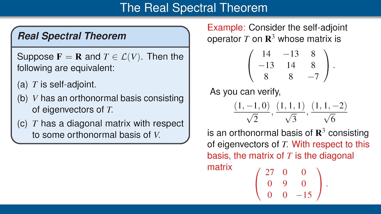
The Spectral Theorem for Complex Hermitian Matrices
A complex $n\times n$ matrix $A$ is Hermitian ($A=A^{†}$) if and only if there exists a unitary matrix $U$ and a real diagonal matrix $D$ such that:
$A=UD{U}^{†}$
The columns of $U$ are an orthonormal basis of eigenvectors for ${\mathbb{C}}^n$, and the diagonal entries of $D$ are the corresponding (real) eigenvalues.

This is a fantastic result! It means that for these important matrices, we can always find a set of perpendicular axes (the eigenvectors) along which the matrix's action is just simple scaling (by the eigenvalues).

2. How to Find the Orthonormal Eigenbasis: The Algorithm

The Spectral Theorem guarantees that an orthonormal basis of eigenvectors exists. Our job is to find it. The process combines what we already know about finding eigenvalues and eigenvectors with the Gram-Schmidt process you learned in Module 3.

Here is a summary of the algorithm:

1. Find the eigenvalues of the symmetric/Hermitian matrix $A$ by solving the characteristic equation $\det (A-\lambda I)=0$.
2. Find a basis for each eigenspace $E_{\lambda }$ by finding the null space of $(A-\lambda I)$.
3. Create an orthonormal basis for each eigenspace:
   • If an eigenspace has dimension 1 (i.e., the eigenvalue is not repeated), simply take the single basis eigenvector and normalize it to have a length of 1.
   • If an eigenspace has dimension $k>1$ (i.e., the eigenvalue is repeated), apply the Gram-Schmidt process to the $k$ basis vectors you found for that eigenspace to get an orthonormal basis for that subspace.
4. Construct the final matrix: The collection of all orthonormal vectors from all the eigenspaces forms the complete orthonormal eigenbasis for the whole space. Create the matrix $Q$ (or $U$) by placing these orthonormal eigenvectors as its columns.

A key point to remember: eigenvectors from different eigenspaces of a symmetric/Hermitian matrix are guaranteed to be orthogonal. You only need to use Gram-Schmidt within an eigenspace if its dimension is greater than one.

3. Worked Examples

Let's apply this algorithm to a few cases.

Example 1: Symmetric Matrix with Distinct Eigenvalues

This is the simplest case. The eigenvectors for the distinct eigenvalues will automatically be orthogonal to each other. We just need to normalize them.

Example 2: Symmetric Matrix with Repeated Eigenvalues

This case is more involved, as it requires the Gram-Schmidt process. Pay close attention to how we create an orthonormal basis for the eigenspace corresponding to the repeated eigenvalue.

Example 3: A Hermitian Matrix

The procedure is identical for Hermitian matrices, but the calculations will involve complex numbers and the complex inner product. This is crucial for your study of quantum mechanics.

4. The Spectral Decomposition: A Deeper Interpretation

The equation $A=Q\Lambda Q^T$ gives us another powerful way to think about symmetric matrices. It can be rewritten as a sum of simple matrices, each representing a projection onto an eigenvector's direction.

The formula is:
$A={\sum }_{i=1}^n{\lambda }_i{q}_i{q}_i^T$
This decomposition is extremely useful. It tells us that the action of any symmetric matrix is a weighted sum of projections onto its orthogonal eigen-directions. The weights are just the eigenvalues.

The following animation provides a beautiful geometric picture of this idea.

Conclusion

This lesson was centered on one of the most elegant and useful theorems in linear algebra. You've not only understood its meaning but also learned the practical steps to apply it.

Key Takeaways:

• The Spectral Theorem guarantees that any real symmetric or complex Hermitian matrix has a full set of eigenvectors that can form an orthonormal basis for the entire space.
• This allows for an orthogonal/unitary diagonalization: $A=Q\Lambda Q^T$ or $A=UD{U}^{†}$.
• We have a concrete algorithm to find this orthonormal basis: find eigenspaces, use Gram-Schmidt within any eigenspace of dimension > 1, normalize all vectors, and combine them.
• The theorem also provides the spectral decomposition, $A=\sum {\lambda }_i{q}_i{q}_i^T$, which interprets the matrix's action as a sum of scaled projections onto its orthonormal eigenvectors.

Preview of the Next Lesson:

We've now fully characterized the eigenvalues and eigenvectors of symmetric matrices. In the next lesson, we will use these results to classify them further. We will define positive definite and semi-definite matrices. This classification is based entirely on the sign of the eigenvalues, a property made accessible by the Spectral Theorem. This concept is fundamental to understanding convex optimization, which is the engine behind training most deep learning models.