Gradient Descent for Multivariate Functions

1. The Intuition: A Ball Rolling Down a Hill

Before diving into the math, let's build a strong mental model. Imagine placing a ball on a hilly landscape. The ball will naturally roll downhill. Gradient descent is the mathematical formalization of this idea. The "landscape" is our function's graph, and the "downhill" direction is determined by the gradient.

The following video provides an excellent high-level intuition for why we want to find a minimum and how gradient descent accomplishes this, all within the context of training a neural network.

As the video explains, the core idea is simple:

1. Start at some point on the function's surface.
2. Find the direction of steepest descent.
3. Take a small step in that direction.
4. Repeat.

The gradient, $\nabla f$, gives the direction of steepest ascent. Therefore, the direction of steepest descent is simply its negative, $-\nabla f$.

2. Formulating the Gradient Descent Algorithm

Let's translate this intuition into a formal algorithm. We want to find the minimum of a multivariate function $f(\mathbf{w})$, where $\mathbf{w}$ is a vector of parameters (e.g., $\mathbf{w}=[w_1,w_2,\dots ,w_n{]}^T$).

The Gradient Descent algorithm is an iterative process defined by the following update rule:

Let's break this down:

• ${\mathbf{w}}_k$ is the vector of parameters at iteration $k$.
• ${\mathbf{w}}_{k+1}$ is the updated vector of parameters for the next iteration.
• $\nabla f({\mathbf{w}}_k)$ is the gradient of the function $f$ evaluated at the current position ${\mathbf{w}}_k$.
• $\eta$ (the Greek letter eta) is the learning rate, a small positive scalar that controls the size of each step.

This rule simply states: "The next position is the current position, minus a small step in the direction of the negative gradient."

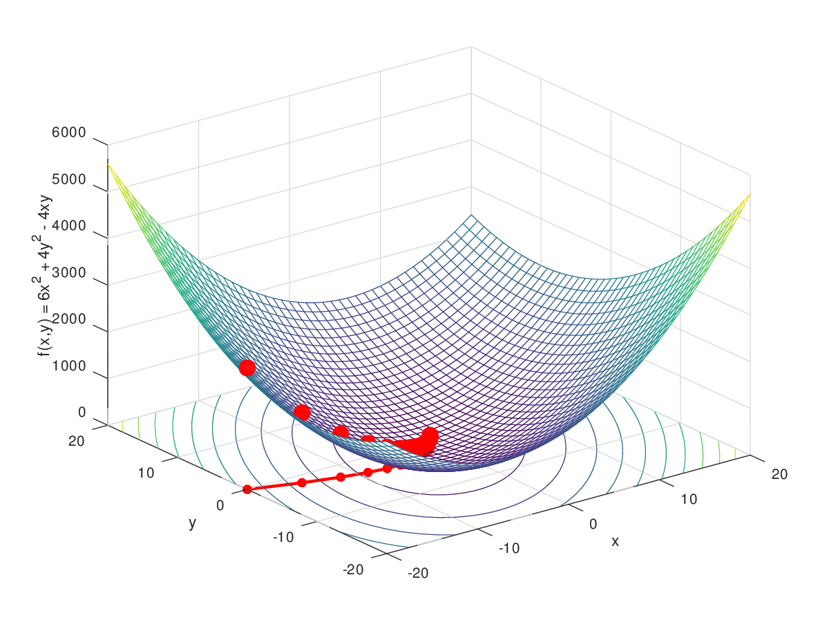
The following video provides a crystal-clear, step-by-step walkthrough of applying this rule, first for a single parameter and then for two parameters, which is exactly what we need for multivariate functions.

3. Key Practical Considerations

The StatQuest video gave you the full mechanical picture. Now, let's focus on a few crucial details that are essential for applying the algorithm correctly.

The Algorithm's Steps

The overall process can be summarized in a simple loop.

The Importance of the Learning Rate ($\eta$)

The learning rate is a critical hyperparameter—a parameter you set before the optimization begins. Its value has a huge impact on performance.

As the reading explains:

• If $\eta$ is too small: The algorithm will take tiny steps, converging very slowly.
• If $\eta$ is too large: The algorithm might "overshoot" the minimum and bounce around, potentially diverging instead of converging.

Finding a good learning rate is often a process of experimentation.

Simultaneous Updates

This is a subtle but critical implementation detail. When you update the parameters in your vector $\mathbf{w}$, you must compute all the components of the gradient first, before changing any of the parameter values.

For example, to update $w_1$ and $w_2$, you would do it like this:

Correct (Simultaneous Update):

1. temp1 = w1 - η * (∂f/∂w1)
2. temp2 = w2 - η * (∂f/∂w2)
3. w1 = temp1
4. w2 = temp2

Note that the calculation for temp2 uses the original w1, not the newly calculated temp1.

4. Applying Gradient Descent: A Worked Example

Let's solidify this by applying the algorithm to a simple convex function: $f(w_1,w_2)=w_1^2+w_2^2$.
We know from our previous lessons that this function is a paraboloid with its minimum at $(0,0)$.

1. Function: $f(w_1,w_2)=w_1^2+w_2^2$
2. Gradient: $\nabla f(\mathbf{w})=\left(\begin{array}{c}\frac{\partial f}{\partial w_1}\\ \frac{\partial f}{\partial w_2}\end{array}\right)=\left(\begin{array}{c}2w_1\\ 2w_2\end{array}\right)$
3. Update Rules:
   • $w_{1,k+1}=w_{1,k}-\eta (2w_{1,k})$
   • $w_{2,k+1}=w_{2,k}-\eta (2w_{2,k})$

Let's choose a starting point ${\mathbf{w}}_0=(3,1)$ and a learning rate $\eta =0.2$.

Iteration 1:

• Current position: ${\mathbf{w}}_0=(3,1)$.
• Calculate gradient at ${\mathbf{w}}_0$: $\nabla f(3,1)=\left(\begin{array}{c}2(3)\\ 2(1)\end{array}\right)=\left(\begin{array}{c}6\\ 2\end{array}\right)$.
• Calculate the step: $\eta \nabla f=0.2\left(\begin{array}{c}6\\ 2\end{array}\right)=\left(\begin{array}{c}1.2\\ 0.4\end{array}\right)$.
• Update position: ${\mathbf{w}}_1={\mathbf{w}}_0-\eta \nabla f=\left(\begin{array}{c}3\\ 1\end{array}\right)-\left(\begin{array}{c}1.2\\ 0.4\end{array}\right)=\left(\begin{array}{c}1.8\\ 0.6\end{array}\right)$.
• Check progress: $f({\mathbf{w}}_0)=3^2+1^2=10$. $f({\mathbf{w}}_1)=1.8^2+0.6^2=3.24+0.36=3.6$. We've moved closer to the minimum!

Iteration 2:

• Current position: ${\mathbf{w}}_1=(1.8,0.6)$.
• Calculate gradient at ${\mathbf{w}}_1$: $\nabla f(1.8,0.6)=\left(\begin{array}{c}2(1.8)\\ 2(0.6)\end{array}\right)=\left(\begin{array}{c}3.6\\ 1.2\end{array}\right)$.
• Calculate the step: $\eta \nabla f=0.2\left(\begin{array}{c}3.6\\ 1.2\end{array}\right)=\left(\begin{array}{c}0.72\\ 0.24\end{array}\right)$.
• Update position: ${\mathbf{w}}_2={\mathbf{w}}_1-\eta \nabla f=\left(\begin{array}{c}1.8\\ 0.6\end{array}\right)-\left(\begin{array}{c}0.72\\ 0.24\end{array}\right)=\left(\begin{array}{c}1.08\\ 0.36\end{array}\right)$.

If we continue this process, the point $(w_1,w_2)$ will get progressively closer to the minimum at $(0,0)$.

Conclusion

Congratulations on completing this crucial lesson! You now understand the mechanics of the primary algorithm that powers much of modern machine learning.

Key Takeaways:

• Gradient Descent is an iterative algorithm for finding the minimum of a function.
• The core update rule is ${\mathbf{w}}_{k+1}={\mathbf{w}}_k-\eta \nabla f({\mathbf{w}}_k)$, which involves taking steps in the direction of the negative gradient.
• The learning rate $\eta$ is a critical hyperparameter that controls step size; if it's too large, the algorithm can diverge, and if it's too small, it will be too slow.
• For multivariate functions, parameter updates must be done simultaneously.

Preview of the Next Lesson:

This was the last lesson in this module, but it sets up the next module perfectly. We have now mastered the tool (Gradient Descent) and the prerequisite calculus. The next step is to apply it to a real-world problem. In our next lesson, we will begin our module on applications by formulating the least squares problem for linear regression. We will define a cost function that measures how well a line fits a set of data points, and then we will use our matrix calculus skills to find the gradient of that cost function—the final piece needed to train a linear regression model using the gradient descent algorithm you learned today.