Eigenvalues and Eigenvectors: Invariant Directions of Linear Transformations

1. The Core Idea: Vectors That Stay on Their Span

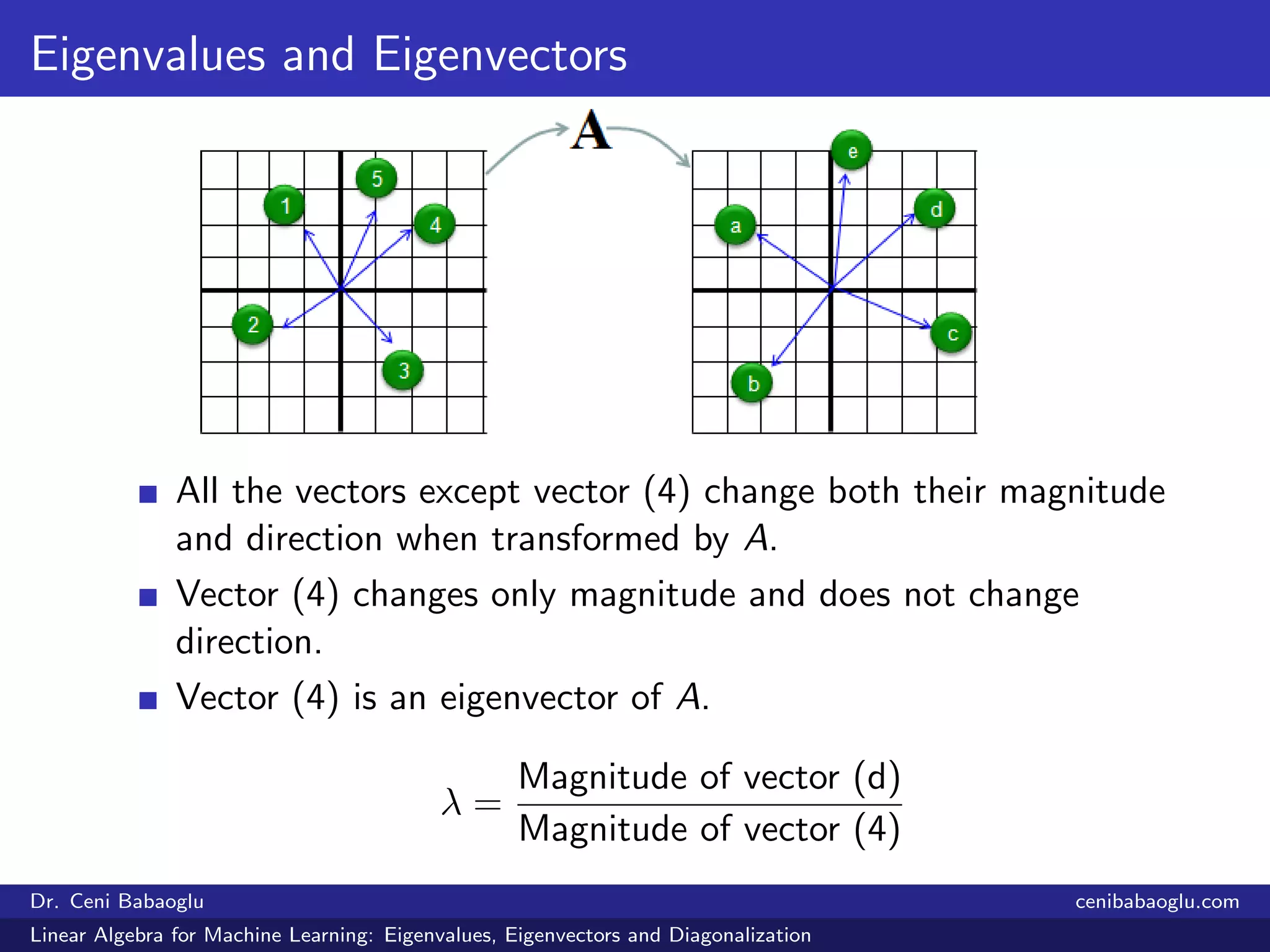
When you apply a linear transformation (i.e., multiply by a matrix), most vectors are knocked off their original direction. Imagine a matrix transformation acting on every vector in a 2D plane. Most vectors will be rotated and stretched, pointing in a new direction.

However, some special vectors might exist that, after the transformation, still point in the same direction (or the exact opposite direction). The transformation only scales them—stretching, squishing, or flipping them. These vectors define the invariant directions of the transformation.

This is the central idea behind eigenvectors.

To formalize what you just saw in the video:

• An eigenvector of a linear transformation is a non-zero vector whose direction is unchanged by the transformation. It remains on its own span.
• The eigenvalue is the scalar factor by which the eigenvector is stretched or shrunk. A negative eigenvalue means the vector is flipped and then scaled.

This relationship is captured by the defining equation of the eigenvalue problem:

Where:

• $A$ is the matrix representing the linear transformation.
• $\mathbf{x}$ is the eigenvector (a non-zero vector).
• $\lambda$ (lambda) is the corresponding eigenvalue (a scalar).

2. Geometric Interpretation Through Examples

The best way to solidify your understanding is to see how eigenvectors and eigenvalues manifest in transformations you're already familiar with.

Example 1: Projection

Consider a projection matrix $P$ that projects vectors onto a plane in 3D space. What are its eigenvectors?

As Professor Strang explained, we can identify two sets of invariant directions for a projection onto a plane:

1. Any vector $\mathbf{x}$ lying in the plane of projection. When you project such a vector, it remains unchanged. Therefore, $P\mathbf{x}=\mathbf{x}$. Comparing this to $P\mathbf{x}=\lambda \mathbf{x}$, we see that these are eigenvectors with an eigenvalue of $\lambda =1$. The entire plane is a space of eigenvectors.
2. Any vector $\mathbf{x}$ perpendicular to the plane of projection. When you project such a vector, it gets mapped to the zero vector. Therefore, $P\mathbf{x}=0$. We can write this as $P\mathbf{x}=0\mathbf{x}$. These are eigenvectors with an eigenvalue of $\lambda =0$. The line perpendicular to the plane is a space of eigenvectors.

Any vector that is not in the plane or perpendicular to it will be an eigenvector. Its direction changes as it is projected onto the plane.

Example 2: 3D Rotation

This example is particularly relevant for your interest in physics. What is the eigenvector of a rotation in 3D?

As the video shows, for a 3D rotation around an axis, the axis of rotation itself is the invariant direction. Any vector lying on this axis will not change its direction during the rotation.

• Eigenvector: Any vector pointing along the axis of rotation.
• Eigenvalue: Since rotation doesn't stretch or shrink vectors, the length remains the same. Thus, the eigenvalue must be $\lambda =1$.

Thinking about a rotation in terms of its axis (eigenvector) and angle is far more intuitive than trying to understand the nine numbers in its 3x3 matrix.

Other Examples

Let's summarize a few other common transformations and their geometric interpretation in terms of eigenvectors.

• Uniform Scaling: If $A=kI$, the matrix scales every vector by a factor of $k$. In this case, every vector in the space is an eigenvector with eigenvalue $\lambda =k$.
• Shear: A shear transformation (like the one in the top right of the image above) "pushes" layers of the space. For a horizontal shear, only vectors on the x-axis stay on their span. They are fixed, so they are eigenvectors with $\lambda =1$.
• 2D Rotation: A rotation in 2D (by an angle other than 0° or 180°) rotates every vector. No vector stays on its span. Therefore, such a transformation has no real eigenvectors. We'll see in the next lesson that this corresponds to finding complex eigenvalues, a concept vital for quantum mechanics.

3. A Glimpse into Finding Eigenvalues

So, how do we find these special values and vectors without relying solely on geometric observation? Let's briefly touch on the algebraic foundation, which we will explore fully in the next lesson.

We start with the defining equation:
$A\mathbf{x}=\lambda \mathbf{x}$

To solve this, we bring everything to one side:
$A\mathbf{x}-\lambda \mathbf{x}=0$
$A\mathbf{x}-\lambda I\mathbf{x}=0$
$(A-\lambda I)\mathbf{x}=0$

This equation is fundamental. It says that an eigenvector $\mathbf{x}$ is a non-zero vector in the null space of the matrix $(A-\lambda I)$.

From our previous work, we know that for a matrix to have a non-zero vector in its null space, the matrix must be singular. And a singular matrix is one whose determinant is zero.

This gives us the crucial condition for finding eigenvalues:
$\det (A-\lambda I)=0$

This is called the characteristic equation. For a given matrix $A$, we can solve this equation to find the possible values of $\lambda$ (the eigenvalues). Once we have an eigenvalue $\lambda$, we can plug it back into $(A-\lambda I)\mathbf{x}=0$ and find the null space to get the corresponding eigenvectors $\mathbf{x}$.

For today, the important takeaway is the connection: the existence of an eigenvector corresponds to the matrix $(A-\lambda I)$ "squishing" space into a lower dimension, which is precisely what $\det (A-\lambda I)=0$ signifies.

Conclusion

In this lesson, we introduced the intuitive, geometric meaning of eigenvalues and eigenvectors. Rather than getting lost in computation, we focused on what they are and what they represent.

Key Takeaways:

• An eigenvector of a transformation is a non-zero vector whose direction is invariant—it stays on its own span.
• An eigenvalue is the scalar factor by which the eigenvector is scaled.
• Geometrically, eigenvectors represent the axes of a transformation. Along these axes, the complex action of a matrix simplifies to simple stretching or shrinking.
• Examples like projections (eigenvalues 1 and 0), reflections (eigenvalues 1 and -1), and 3D rotations (eigenvalue 1 for the axis of rotation) highlight this geometric role.
• The algebraic condition for an eigenvalue $\lambda$ to exist is that the matrix $(A-\lambda I)$ must be singular, leading to the characteristic equation $\det (A-\lambda I)=0$.

Preview of the Next Lesson:

We've built the geometric foundation. In the next lesson, we will get our hands dirty with the algebra. You will learn the systematic process to compute the characteristic polynomial to find eigenvalues and their corresponding eigenvectors. We will move from identifying invariant directions visually to calculating them precisely for any given matrix.