Singular Values and Vectors

1. The SVD Equation: A First Look

The Singular Value Decomposition states that any $m\times n$ matrix $A$ can be factored into the product of three other matrices:

$A=U\Sigma V^T$

This decomposition breaks down the action of the matrix $A$ into three fundamental components. Let's get acquainted with them.

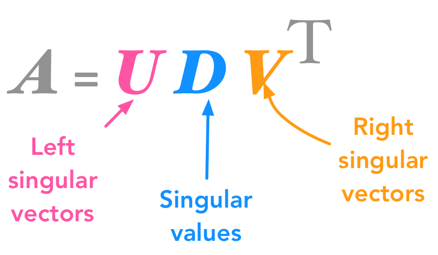
The video below gives a great high-level introduction to these three matrices and their properties.

As the video explains, the components are:

• $U$: An $m\times m$ orthogonal matrix. Its columns are called the left singular vectors.
• $\Sigma$: An $m\times n$ rectangular diagonal matrix. The non-negative diagonal entries, denoted ${\sigma }_i$, are called the singular values. They are ordered from largest to smallest: ${\sigma }_1\ge {\sigma }_2\ge \cdots \ge 0$.
• $V$: An $n\times n$ orthogonal matrix. Its columns are called the right singular vectors. Note that the formula uses its transpose, $V^T$.

This structure should feel somewhat familiar. It resembles the $PD{P}^T$ decomposition, but with two different orthogonal matrices ($U$ and $V$) instead of just one ($P$). This is what gives SVD the flexibility to work for any matrix.

2. The Geometric Meaning of SVD

The real power of SVD comes from its geometric interpretation. It tells us that any linear transformation can be decomposed into a sequence of three simple operations:

1. A rotation (and/or reflection) in the input space.
2. A scaling along the coordinate axes.
3. A rotation (and/or reflection) in the output space.

The following resource provides a fantastic, jargon-free explanation of this idea.

Here's how the matrices from the SVD equation map to this geometric picture:

• $V^T$ performs the initial rotation in the input space.
• $\Sigma$ performs the scaling. The singular values ${\sigma }_i$ are the scaling factors along each axis.
• $U$ performs the final rotation in the output space.

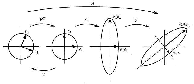
The singular vectors and values have a precise relationship that defines this transformation. For each right singular vector $v_i$ and corresponding left singular vector $u_i$, the matrix $A$ transforms $v_i$ into a scaled version of $u_i$:

$A{\mathbf{v}}_i={\sigma }_i{\mathbf{u}}_i$

This is a central equation in SVD. It's similar to the eigenvector equation $A\mathbf{x}=\lambda \mathbf{x}$, but here the input vector (${\mathbf{v}}_i$) and output vector (${\mathbf{u}}_i$) are from different orthogonal bases. The SVD finds the special orthonormal basis in the input space ($\{{\mathbf{v}}_i\}$) that gets mapped to an orthogonal basis in the output space ($\{{\mathbf{u}}_i\}$), with the only coupling being the scaling factors ${\sigma }_i$.

3. A Constructive Definition: The Link to Eigenvalues

So far, we've defined the singular vectors and values as parts of the SVD equation. But how are they actually found? This gives us a more concrete, constructive definition. The key is to create a symmetric matrix from $A$, which allows us to use the tools from our previous module.

Consider the matrix $A^{T}A$. If $A=U\Sigma V^T$, then:
$A^{T}A=(V{\Sigma }^T{U}^T)(U\Sigma V^T)$
Since $U$ is orthogonal, $U^{T}U=I$. This simplifies to:
$A^{T}A=V({\Sigma }^T\Sigma )V^T$
This is the eigenvalue decomposition of the symmetric matrix $A^{T}A$! This tells us:

• The right singular vectors (columns of $V$) are the eigenvectors of $A^{T}A$.
• The singular values (${\sigma }_i$) are the square roots of the eigenvalues of $A^{T}A$. (${\lambda }_i={\sigma }_i^2$).

Similarly, if we look at $A{A}^T$:
$A{A}^T=(U\Sigma V^T)(V{\Sigma }^T{U}^T)=U(\Sigma {\Sigma }^T)U^T$
This tells us:

• The left singular vectors (columns of $U$) are the eigenvectors of $A{A}^T$.

The following video with Professor Strang explains this derivation clearly.

4. An Alternative Viewpoint: Directions of Maximum "Action"

There's another powerful way to define singular vectors that is especially useful in data science. Instead of starting with the decomposition, we can define the singular vectors greedily.

Imagine you have a cloud of data points represented by the rows of matrix $A$. You want to find the direction in space (a unit vector $\mathbf{v}$) such that when you project all your data points onto it, the sum of the squared projection lengths is maximized. This direction is the "most important" direction in your data.

It turns out:

• The first right singular vector ${\mathbf{v}}_1$ is precisely this direction: ${\mathbf{v}}_1=\arg {\max }_{|\mathbf{v}|=1}|A\mathbf{v}|$.
• The first singular value ${\sigma }_1$ is the value of this maximum: ${\sigma }_1=|A{\mathbf{v}}_1|$.
• The second right singular vector ${\mathbf{v}}_2$ is the direction, orthogonal to ${\mathbf{v}}_1$, that maximizes $|A\mathbf{v}|$.
• And so on.

This approach defines the singular vectors and values in order of importance, which is a key reason why SVD is so useful for data compression and analysis.

Conclusion

In this lesson, we have introduced the Singular Value Decomposition and defined its core components. While we've approached it from several angles, they all describe the same fundamental structure.

Key Takeaways:

• Any matrix $A$ can be decomposed as $A=U\Sigma V^T$, where $U$ and $V$ are orthogonal matrices and $\Sigma$ is a diagonal matrix of singular values.
• The columns of $U$ are the left singular vectors, which are the eigenvectors of $A{A}^T$.
• The columns of $V$ are the right singular vectors, which are the eigenvectors of $A^{T}A$.
• The diagonal entries of $\Sigma$ are the singular values (${\sigma }_i$), which are the square roots of the eigenvalues of $A^{T}A$ (or $A{A}^T$).
• Geometrically, SVD decomposes any linear transformation into a rotation ($V^T$), a scaling by the singular values ($\Sigma$), and another rotation ($U$).
• The relationship $A{\mathbf{v}}_i={\sigma }_i{\mathbf{u}}_i$ connects the singular vectors and values, showing how $A$ maps one orthonormal basis to another.

Preview of the Next Lesson:

We now know what the singular values and vectors are. In the next lesson, we will put this knowledge into practice and construct the full and reduced Singular Value Decomposition of a matrix. We'll work through a concrete example from start to finish, using the eigenvalue-based method we learned about today.