Hello! Welcome to the fourth lesson in our module on understanding AI performance metrics.
In our last lesson, we discovered why overall accuracy can be a deceptive metric. You learned that in clinical situations with imbalanced data—like screening for a rare disease—a model can achieve a very high accuracy score while being completely useless for its primary task. This is because accuracy treats all errors as equal, but clinically, missing a real disease (a false negative) is often far more serious than flagging a healthy patient for a follow-up (a false positive).
This highlights the need for a more sophisticated tool to evaluate diagnostic models. We need a way to see the full picture of a model's performance, not just a single, potentially misleading number.
That brings us to today's goal: to interpret a Receiver Operating Characteristic (ROC) curve and the meaning of the Area Under the Curve (AUC). These are among the most common tools you will encounter when reading AI research in dentistry, and understanding them is essential for assessing a model's true diagnostic capability.
The Threshold Problem
Most AI diagnostic models don't just give a 'yes' or 'no' answer. Instead, they output a probability or a confidence score. For example, an AI analyzing a bitewing radiograph might report a "73% probability of an interproximal carious lesion."
As a user or developer, you have to set a threshold to turn that probability into a clinical decision.
- If you set a low threshold (e.g., >20%), you'll be very sensitive, catching almost every potential lesion. However, you'll also have many false positives.
- If you set a high threshold (e.g., >90%), you'll be very specific, and any lesion you flag will very likely be real. But you'll miss many of the more subtle, early-stage lesions (high false negatives).
So, which threshold is best? The ROC curve is a tool that helps us answer this by showing the performance across all possible thresholds at once.
Visualizing the Trade-off: The ROC Curve
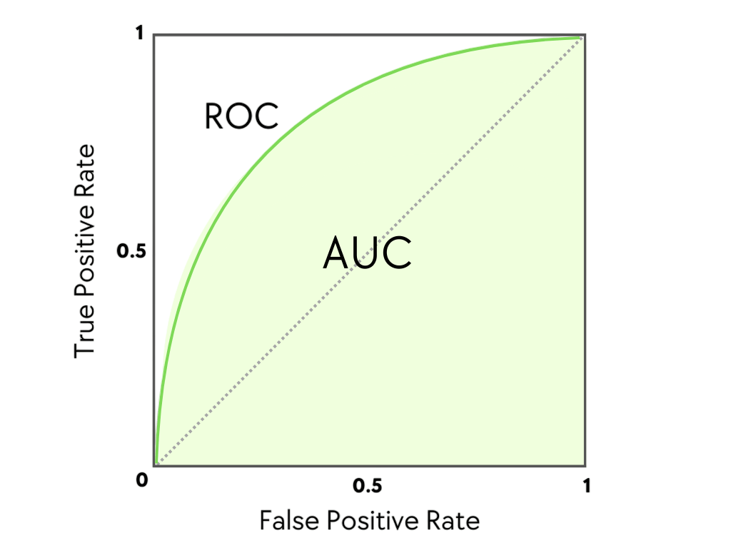
An ROC curve is a graph that plots the trade-off between the benefits of a test (correctly identifying disease) and its costs (incorrectly flagging healthy individuals).
The axes of an ROC curve are:
- Y-axis: True Positive Rate (TPR), which is another name for Sensitivity. It answers: "Of all the people who actually have the disease, what fraction did the test correctly identify?"
- X-axis: False Positive Rate (FPR), which is calculated as (1 - Specificity). It answers: "Of all the people who are healthy, what fraction did the test incorrectly flag as diseased?"
To see how this graph is built and what it represents in a clinical context, let's watch a clear explanation from a physician's perspective.
In this video, 'How to interpret ROC curves,' Dr. Terry Shaneyfelt explains the concept of diagnostic test cut-offs and how they are used to construct an ROC curve.
Watch the sections from 00:41 to 02:51. First, focus on the explanation of how changing a cut-off point affects false positives and false negatives (00:41-01:48). Then, pay close attention to how the curve is constructed by plotting sensitivity against (1 - specificity) for each of these points (01:59-02:51).
How to Read an ROC Curve
As you saw in the video, an ROC curve has a few key features that tell you about the quality of the test:
- The Diagonal Line (Line of No Discrimination): A straight diagonal line from the bottom-left corner (0,0) to the top-right corner (1,1) represents a test that is no better than a random guess, like flipping a coin. On this line, the True Positive Rate is always equal to the False Positive Rate.
- The Top-Left Corner (The "Perfect" Test): The point (0,1) represents a perfect test with 100% sensitivity (it catches every disease case) and 100% specificity (it produces zero false alarms).
- The Curve: The closer the ROC curve "bows" toward the top-left corner, the better the diagnostic test. A better test gives you a higher True Positive Rate for any given False Positive Rate.
This makes ROC curves excellent for comparing different diagnostic tests.

Summarizing Performance: The Area Under the Curve (AUC)
While the curve gives you a visual representation, it's often useful to have a single number to summarize the overall performance of the test. This is the Area Under the Curve (AUC).
The AUC represents the probability that the model will rank a randomly chosen positive instance higher than a randomly chosen negative one. In simpler terms, it's a measure of the test's ability to distinguish between diseased and healthy patients.
- An AUC of 1.0 represents a perfect test.
- An AUC of 0.5 represents a worthless test (the diagonal line).
- A real-world diagnostic test will have an AUC between 0.5 and 1.0.
Let's return to Dr. Shaneyfelt's video to see how he explains AUC and uses it to compare multiple tests.
First, watch from 02:51 to 03:24 to get a clear definition of AUC as a measure of overall accuracy. Then, watch from 04:17 to 05:02, where he shows how to use AUC scores to compare the performance of three different diagnostic tests for the same condition.
The AUC gives us a much more robust measure of a model's performance than overall accuracy because it is not dependent on a single chosen threshold and is less affected by imbalanced datasets.
Here is a common rule of thumb for interpreting AUC values in a clinical context:
| Area under the Curve (AUC) | Interpretation |
|---|---|
| 0.90 – 1.00 | Excellent |
| 0.80 – 0.90 | Good |
| 0.70 – 0.80 | Fair |
| 0.60 – 0.70 | Poor |
| 0.50 – 0.60 | Fail / No Discrimination |
This table provides a quick way to judge the quality of an AI model you might read about in a research paper.
For a more formal and detailed definition, you can refer to this article from the Journal of the Canadian Dental Association.
[PDF] Part 2. Using Predictive Values and Receiver Operating ...
This article provides a formal, text-based summary of ROC curves and AUC, reinforcing what we've seen in the videos.
Read the section titled 'Area under the Curve'. It clearly defines AUC as a summary index of discriminatory accuracy and explains the 0.5 to 1.0 scale.
From Potential to Practice: Choosing an Operating Point
The AUC tells you about the overall potential of a diagnostic test. However, to use the test in practice, you still need to choose a single threshold, which corresponds to a single point on the ROC curve.
The "best" point to choose depends entirely on the clinical context.
- For a screening test for a dangerous but treatable disease (like oral cancer), you want to maximize sensitivity to avoid missing any cases. You would choose a point on the curve that is high up on the y-axis, even if it means moving a bit to the right on the x-axis (accepting more false positives).
- For a confirmatory test before an invasive or expensive treatment (like a biopsy), you want to maximize specificity to avoid treating healthy patients. You would choose a point on the curve that is far to the left on the x-axis, even if it means sacrificing some sensitivity.
This video provides an excellent summary of these concepts.
USMLE Step 1 Biostatistics and Epidemiology - Receiver operating curves (ROC curves)
This video, aimed at medical students, recaps the ROC curve and AUC and then directly addresses how clinical goals influence the choice of a cut-off point.
Watch from 02:47 to 04:10. Pay close attention to the discussion on when to prioritize a test with high sensitivity versus one with high specificity, based on the clinical scenario.
Conclusion
You have now learned how to interpret one of the most important tools for evaluating diagnostic AI. Unlike overall accuracy, the ROC curve and its corresponding AUC value give you a comprehensive and reliable view of a model's performance.
Key Takeaways:
- An ROC curve plots the True Positive Rate (Sensitivity) against the False Positive Rate (1 - Specificity) across all possible thresholds.
- A test is better when its curve bows closer to the top-left corner. A test on the diagonal line is no better than a random guess.
- The Area Under the Curve (AUC) is a single number from 0.5 (useless) to 1.0 (perfect) that summarizes the overall diagnostic ability of a test.
- AUC is a more robust metric than accuracy, especially for the imbalanced datasets common in dentistry.
- While AUC measures a model's overall potential, the choice of a specific operating threshold on the curve is a clinical decision that depends on the trade-off between sensitivity and specificity.
In our next and final lesson for this module, we will dive deeper into this last point. We will focus on how to relate performance metrics to clinical utility, exploring case studies where you might choose a high-sensitivity model over a high-specificity one, or vice-versa, in a dental setting.