Hello! Welcome to the first lesson in our new module, Unsupervised Learning & Dimensionality Reduction.
In the previous module, we focused on supervised learning, where we trained models using data that had known correct answers or labels (e.g., classifying an email as spam or not spam). We concluded by looking at the structure of neural networks, which are powerful models for complex supervised tasks.
Now, we pivot to unsupervised learning. What if you have a dataset with no labels at all? The goal here isn't to predict a known outcome, but to discover hidden structures, patterns, or groupings within the data itself. One of the most fundamental tasks in unsupervised learning is clustering.
Today's lesson addresses the learning outcome: Explain partitioning clustering algorithms (k-means/k-medoids). We will explore two of the most widely-used algorithms that partition data into a specified number of groups. This is a foundational topic in data science and frequently appears on exams like the GATE.
1. What is Partitioning Clustering?
Imagine you have a scatter plot of data points, and you want to group them into distinct "clouds" or clusters. Partitioning algorithms do exactly this: they divide the dataset into a pre-determined number of non-overlapping groups. The "pre-determined number" is a key parameter, which we'll call . Our goal is to create clusters where points within a cluster are very similar to each other, and points in different clusters are dissimilar.
2. K-Means Clustering: Grouping by the Mean
K-Means is arguably the most famous and widely used clustering algorithm due to its simplicity and speed. The core idea is to represent each cluster by its center, called a centroid, which is the mean of all the data points in that cluster.
The following video from StatQuest provides an excellent, intuitive explanation of how the K-Means algorithm works iteratively to find these clusters.
This video, 'StatQuest: K-means clustering', will walk you through the entire K-Means process, from initialization to convergence.
Watch the segment from 01:04 to 04:23. Focus on understanding the two repeating steps: (1) assigning points to the nearest cluster center and (2) updating the cluster center to be the new mean.
As the video demonstrated, the K-Means algorithm follows these simple, iterative steps:
- Initialize: Choose the number of clusters, . Then, randomly select data points from your dataset to serve as the initial centroids.
- Assign: For each data point, calculate its distance to every centroid (typically using Euclidean distance). Assign the data point to the cluster of the nearest centroid.
- Update: Recalculate the centroid of each cluster by taking the mean of all data points assigned to it.
- Repeat: Keep repeating the Assign and Update steps until the centroids no longer move significantly, meaning the cluster assignments have stabilized.
How to Choose the Right ?
A critical question is how to determine the number of clusters, . The "Elbow Method" is a common heuristic for this. You run K-Means for a range of values and plot the within-cluster sum of squares (WCSS) for each. The WCSS measures the total variance within all clusters.
Let's return to the StatQuest video to see how the Elbow Method works.
Watch the segment from 04:23 to 06:13. Notice how the plot of variation vs. number of clusters forms an 'elbow'. This point of inflection is often a good choice for k.
The intuition is that as increases, the WCSS will always decrease. However, after a certain point (the "elbow"), adding more clusters doesn't significantly reduce the total variation. This point suggests a natural grouping in the data.
3. K-Medoids Clustering: A More Robust Alternative
K-Means is fast and effective, but it has a weakness: the cluster centroids are calculated as the mean of the points. If your cluster contains outliers (extreme values), the mean can be pulled far away from the natural center of the cluster.
K-Medoids solves this problem. Instead of a centroid, it uses a medoid to represent the cluster. A medoid is an actual data point in the cluster that is the most centrally located.
This simple change makes the algorithm much more robust to outliers.

The K-Medoids algorithm, often called Partitioning Around Medoids (PAM), works as follows:
- Initialize: Choose and randomly select data points as the initial medoids.
- Assign: Assign each data point to the cluster of its closest medoid.
- Update: This is the clever part. For each cluster, the algorithm iteratively swaps one of the medoids with a non-medoid point in the dataset. It calculates the total cost (e.g., the sum of distances of all points to their medoid) for this new configuration. If the swap reduces the total cost, it is kept.
- Repeat: This swapping process continues until no swap can further reduce the total cost.
The following video explains this iterative swapping process.
K-Medoid Clustering Algorithm | K-Medoids Clustering Algorithm | K-Medoids Clustering Mahesh Huddar
This video, 'K-Medoid Clustering Algorithm', explains the step-by-step process, focusing on the cost calculation and swapping step.
Watch from 00:51 to 06:57. The key is to understand the idea of calculating a 'total cost' for a set of clusters and then trying to improve it by swapping medoids.
4. K-Means vs. K-Medoids: Key Differences for the Exam
For your GATE preparation, it's crucial to know when to use each algorithm. The choice boils down to a trade-off between robustness and computational efficiency.
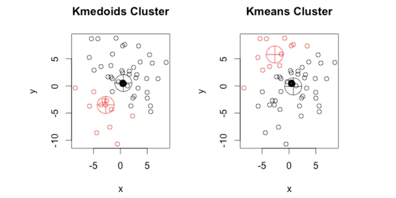
The following article provides a concise summary of the practical differences. The comparison table is especially useful for revision.
Difference between K means and K medoids Clustering
The GeeksforGeeks article 'Difference between K means and K medoids Clustering' provides a direct comparison of the two algorithms. This is perfect for creating quick revision notes.
Read the sections 'Key Differences Between K-Means and K-Medoids' and 'Practical Considerations'. Focus on the table that summarizes the differences in representation, outlier sensitivity, distance metrics, and efficiency.
Here is a summary of the most important distinctions:
| Aspect | K-Means | K-Medoids |
|---|---|---|
| Cluster Center | Centroid: The mean of the points in the cluster. May not be an actual data point. | Medoid: The most centrally located data point within the cluster. |
| Outlier Sensitivity | High. Outliers can significantly skew the centroid. | Low. Since the medoid must be an actual point, it is less affected by outliers. |
| Computational Cost | Lower. Calculating the mean is fast. | Higher. Iteratively swapping and re-calculating costs for all points is expensive. |
| Use Case | Good for large datasets where efficiency is key and clusters are roughly spherical. | Good for datasets with noise and outliers, or when the mean is not a meaningful center. |
Conclusion
In this lesson, we explored our first unsupervised learning task: clustering. We focused on partitioning algorithms, which divide data into a pre-specified number of groups, .
Key Takeaways:
- Partitioning clustering aims to divide data into non-overlapping clusters.
- K-Means uses the mean of points (centroid) as the cluster center. It is fast but sensitive to outliers.
- K-Medoids uses an actual data point (medoid) as the cluster center. It is robust to outliers but computationally more expensive.
- The choice between them involves a trade-off between robustness (K-Medoids) and speed (K-Means).
- The Elbow Method is a common heuristic to help choose an appropriate value for .
Preview of the Next Lesson:
While partitioning algorithms are powerful, they require you to specify in advance. What if you don't know how many clusters to expect? In our next lesson, we will explore a different approach: Explain hierarchical clustering and how to interpret dendrograms. This method builds a nested hierarchy of clusters, which can be visualized as a tree, offering a more exploratory view of your data's structure.