Understanding PCA for Dimensionality Reduction

1. The Core Idea: Finding a Better Perspective

Imagine you have a dataset with many features. Trying to visualize the relationships between them by plotting every pair of features would be overwhelming and often uninformative. PCA provides a way to summarize this high-dimensional data in a much smaller number of dimensions, typically two or three, for visualization and analysis.

The following short video gives an excellent high-level overview of why we need PCA and what it accomplishes.

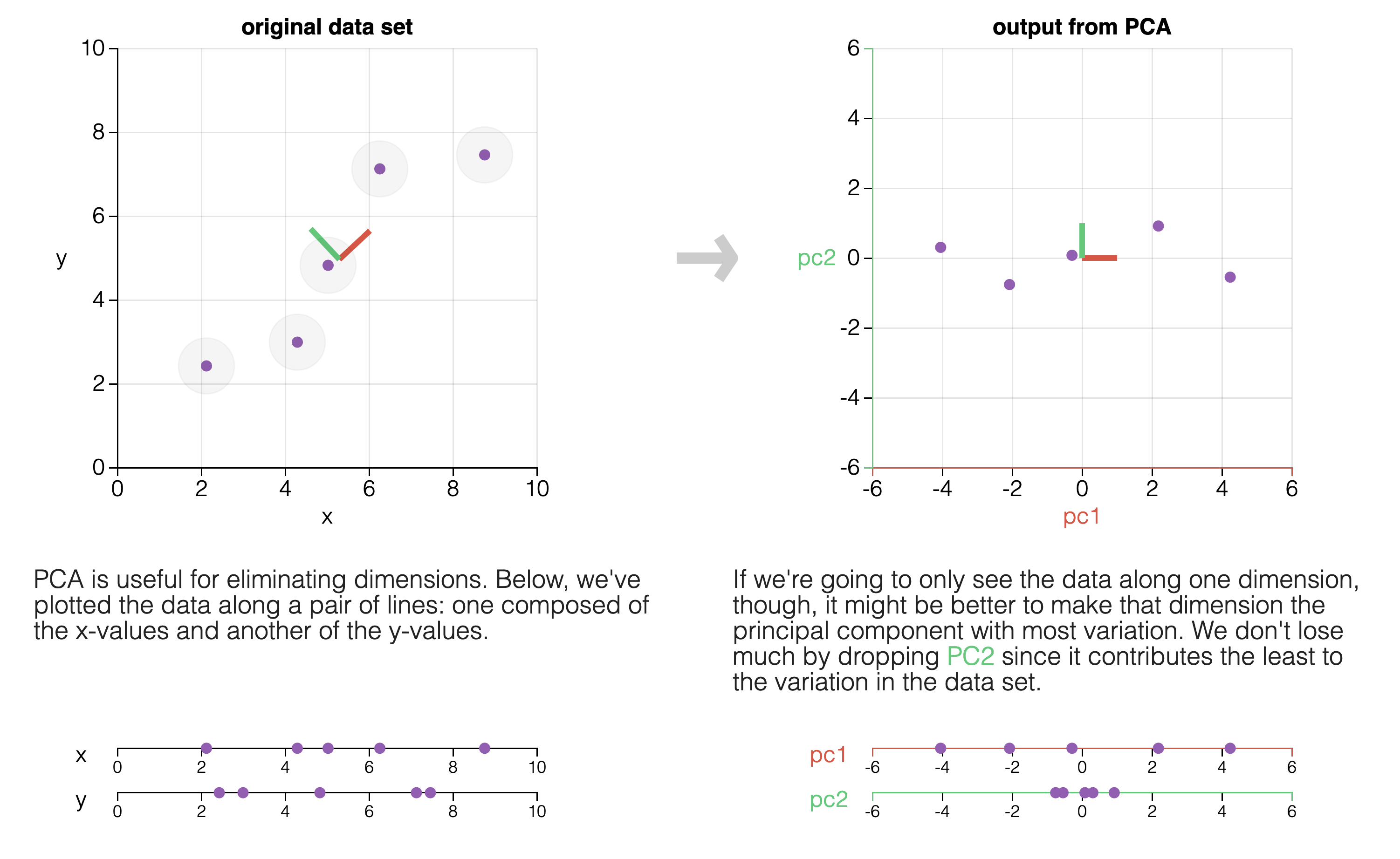
As the video explained, PCA creates new variables called Principal Components (PCs). The key idea is that PCA performs a rotation of the coordinate axes to find a new coordinate system. The new axes are chosen to point in the directions of maximum variance in the data.

2. How PCA Finds the Principal Components

Now that you have the main idea, let's briefly touch upon how PCA finds these new axes. While the underlying math involves linear algebra concepts like eigenvectors, you primarily need to understand the process intuitively for the GATE exam.

The process can be summarized in these conceptual steps:

1. Standardize the Data: PCA is sensitive to the scale of the original variables. If one feature (e.g., salary in rupees) has a much larger range than another (e.g., years of experience), it will dominate the analysis. To prevent this, all features are first standardized to have a mean of 0 and a standard deviation of 1.

2. Find the First Principal Component (PC1): PCA finds a new axis (a line) that passes through the centered data such that when the data points are projected onto this line, the variance of the projected points is maximized. This line is Principal Component 1 (PC1). It represents the single direction that captures the most variability in the dataset.

3. Find the Second Principal Component (PC2): PCA then finds a second axis, Principal Component 2 (PC2), that is orthogonal (perpendicular) to PC1 and captures the maximum remaining variance.

4. Continue for all Dimensions: This process continues, with each subsequent principal component being orthogonal to all previous ones and capturing the maximum possible remaining variance. You will have as many principal components as you have original features.

The following article provides a clear, step-by-step walkthrough of this process. Focus on understanding the logic of each step rather than memorizing the formulas.

Connecting to Your Linear Algebra Background

As the article mentioned, the principal components are mathematically the eigenvectors of the data's covariance matrix. The amount of variance captured by each principal component is its corresponding eigenvalue.

• Eigenvectors define the direction of the new axes (the principal components).
• Eigenvalues measure the magnitude or importance of these directions (the amount of variance along that axis).

By ranking the eigenvectors by their corresponding eigenvalues from largest to smallest, you get the principal components in order of significance: PC1, PC2, PC3, and so on.

3. Using PCA: How Many Components Should You Keep?

Since the goal of PCA is dimensionality reduction, we usually don't want to keep all the principal components. We want to keep a smaller number of components that still capture a large percentage of the total information (variance) in the original data.

So, how do we decide how many to keep? We use a tool called a scree plot.

A scree plot shows the percentage of variance explained by each principal component, ordered from the most important to the least important.

The following video segment explains this perfectly.

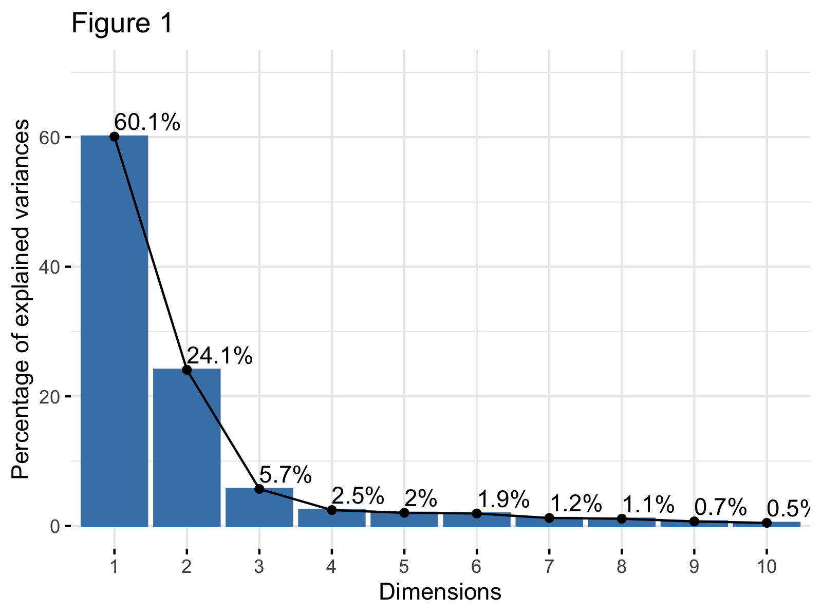
There are two common ways to use a scree plot to decide how many components to keep:

1. The Elbow Method: Look for an "elbow" in the plot where the curve flattens out. The components before the elbow are the ones that explain the most variance. In the plot above, the elbow occurs around the third component, suggesting that keeping 2 or 3 components might be optimal.
2. Cumulative Variance Threshold: Decide on a threshold for the total variance you want to retain (e.g., 90% or 95%). Add up the explained variance of each component until you reach that threshold. In the example above, to get 90% of the variance, you would need to keep the first three components (60.1% + 24.1% + 8.9% ≈ 93%).

4. Advantages and Disadvantages of PCA

Like any technique, PCA has its trade-offs. It's important to know when it is most useful.

Key Advantages:

• Reduces Dimensionality: Simplifies data, which can make subsequent machine learning algorithms faster and more effective.
• Removes Redundancy: The new principal components are uncorrelated, removing multicollinearity between features.
• Noise Reduction: By discarding components with low variance, you can often filter out noise in the data.

Key Disadvantages:

• Interpretability: The principal components are linear combinations of the original features. This makes them less interpretable than the original features. For example, PC1 might be 0.7 * height - 0.3 * weight + 0.1 * age, which doesn't have a clear real-world meaning.
• Information Loss: By discarding some components, you inevitably lose some information.
• Assumes Linearity: PCA is based on linear transformations and may not perform well if the underlying data structure is highly non-linear.

Conclusion

In this lesson, we demystified Principal Component Analysis, one of the most important techniques for dimensionality reduction in machine learning.

Key Takeaways:

• PCA is an unsupervised learning technique used to reduce the number of features in a dataset by transforming them into a new set of uncorrelated variables called Principal Components.
• The principal components are ordered by the amount of variance they explain. PC1 captures the most variance, PC2 captures the second most, and so on.
• Mathematically, the PCs are the eigenvectors of the data's covariance matrix, and the amount of variance they capture is given by the eigenvalues.
• A scree plot is used to visualize the variance explained by each component and helps decide how many components to retain for analysis.
• While PCA is powerful for simplifying data and improving model performance, its main drawback is that the resulting components can be difficult to interpret.

Preview of the Next Lesson:
This lesson concludes our module on Unsupervised Learning and Dimensionality Reduction. We are now moving into the final module of this crash course: AI Concepts: Search and Reasoning. In the next lesson, we will shift gears from analyzing data structure to exploring foundational algorithms for problem-solving. We will begin with "Describe graph traversal (BFS, DFS) and shortest path algorithms (Dijkstra's)," which are essential for navigating and finding solutions in complex, state-based problems.