Welcome to the final lesson of our course!
In our previous session, we established the foundations of knowledge representation using formal logic. We saw how propositional and predicate logic allow an AI to represent and reason about facts that are definitively true or false. However, the real world is rarely so certain. This brings us to the final topic of our AI module and the entire course.
This lesson addresses the learning outcome: Explain the core ideas of reasoning under uncertainty (conditional independence, inference). We will explore how AI systems can represent and reason about knowledge that is probabilistic, using a powerful tool called Bayesian Networks. We'll learn how these networks are built on the concept of conditional independence and how we can query them using exact and approximate inference techniques.
1. From Certainty to Uncertainty: The Need for Probabilistic Reasoning
In our last lesson, we could make a statement like ∀x Man(x) → Mortal(x) ("All men are mortal"). This is a hard, certain rule. But what about a statement like "If a patient has a fever, they might have the flu"? The word "might" introduces uncertainty.
A full joint probability distribution table, which lists the probability of every possible combination of variable states, is the most basic way to represent this uncertainty. However, for binary variables, this table has entries, which becomes computationally impossible to store and use for even a modest number of variables.
The solution is to find a more compact way to represent this joint distribution. This is achieved using Bayesian Networks, which exploit the concept of conditional independence.
These notes from GeeksforGeeks provide a concise introduction to the core concepts we'll be discussing. They are an excellent reference for your GATE preparation.
Please read the first section titled 'Reasoning Under Uncertainty', focusing on the parts about 'Bayesian Networks' and 'Conditional Independence'. Notice how the example Rain→WetGrass←Sprinkler illustrates that rain and the sprinkler are independent before we know if the grass is wet.
2. Bayesian Networks and Conditional Independence
A Bayesian Network (or Bayes Net) is a directed acyclic graph (DAG) that represents a joint probability distribution.
- Nodes: Each node represents a random variable.
- Edges (Arrows): An arrow from node X to node Y means that X is a "parent" of Y, and it directly influences Y.
- Conditional Probability Tables (CPTs): Each node has a CPT that quantifies the probability of that node's state given the states of its parents.
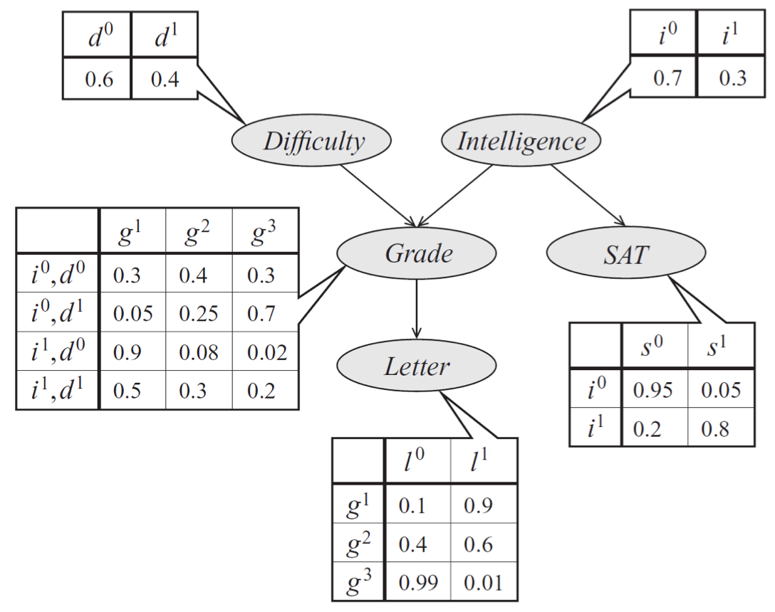
The power of a Bayes Net comes from the fact that it encodes conditional independence assumptions. A node is conditionally independent of all its non-descendants, given its parents. This allows us to factorize the full joint probability distribution into a product of local conditional probabilities from the CPTs.
For the network above, the full joint probability is:
This is far more compact than a giant table for all five variables.
To build a deeper intuition for conditional independence, it helps to understand the three fundamental structures in a Bayes Net.
Probabilistic Reasoning - IIT Delhi
These lecture slides from IIT Delhi clearly explain the three key structures that determine conditional independence in a Bayesian Network.
Read the section titled 'Bayesian Network: Independence Assumptions' (slides 47-56). Focus on understanding the three cases: Causal Chains (A → B → C): Influence flows unless B is observed. Common Cause (A ← B → C): Influence flows unless B is observed. Common Effect (A → B ← C): Influence is blocked unless B (or a descendant of B) is observed. This is often called a v-structure and is a key concept.
3. Inference: Asking Questions to a Bayesian Network
Once we have a Bayes Net, we can use it to answer probabilistic questions. This process is called inference. The general form of a query is to find the posterior probability of some query variable(s) , given some observed evidence variable(s) : .
Variables that are not in the query or the evidence are called hidden variables. To answer a query, we need to sum out (or marginalize) these hidden variables.
There are two main approaches to inference: exact and approximate.
3.1. Exact Inference: Variable Elimination
Exact inference algorithms compute the precise probability for a query. The most fundamental method is Variable Elimination.
The naive approach, "inference by enumeration," involves calculating the full joint distribution and then summing out the hidden variables. As we've discussed, this is highly inefficient. Variable Elimination is a much smarter dynamic programming algorithm that avoids this.
Core Idea: Instead of creating one huge factor by joining all variables and then summing out the hidden ones, Variable Elimination interleaves these operations. It eliminates hidden variables one by one, creating smaller intermediate factors along the way. The key is to push the summations as far inside the expression as possible to minimize the size of the tables you have to compute.
To see why this is so much more efficient, let's watch a video that compares the number of calculations needed with and without Variable Elimination.
Exact Inference using Variable Elimination Algorithm | Lec-7 AI | Anshul Sir | MindMatrix Learning
This video from MindMatrix Learning provides a fantastic motivation for using the Variable Elimination algorithm by demonstrating the computational savings.
Watch the segment from 33:23 to 48:00. The instructor walks through calculating the number of addition and multiplication operations for a query using the full joint distribution versus using the Variable Elimination approach. Focus on the core takeaway: rearranging the summations and products drastically reduces the number of operations from 47 to 14 in this example. This demonstrates why the algorithm is so important.
As the video shows, by reordering operations, Variable Elimination avoids creating massive intermediate tables, making exact inference feasible for many networks.
For your notes, the GATE DA Short Notes - AI (resource LINK, section 1) has a great summary table of the Variable Elimination steps.
3.2. Approximate Inference: Sampling
Why do we need it? For very large or densely connected (loopy) networks, even Variable Elimination becomes computationally intractable (it's an NP-hard problem). In these cases, we resort to approximate inference.
The core idea is to generate a large number of random samples from the distribution and use the frequencies of those samples to estimate the probability we're interested in. These are often called Monte Carlo methods.
Let's explore the high-level idea and the main sampling algorithms you need to know for the GATE exam.
Artificial Intelligence 10 | Approximate Inference through Sampling | DA | GATE Crash Course
This video from GeeksforGeeks explains why we need approximate inference and introduces the core concepts of sampling-based methods.
Please watch the following segments: Why Approximate Inference? (03:16 - 09:26): This part explains that sampling is used when exact methods are too complex or slow. It introduces the idea of generating samples to match a scenario and predict an outcome. Likelihood Weighting (09:26 - 13:10): This explains the Likelihood Weighting algorithm. The key idea is to fix the evidence variables, sample the non-evidence variables, and assign a weight to each sample based on how likely the evidence was, given its parents. The weight is calculated as w = w imes P( ext{evidence_variable} | ext{Parents}). Rejection Sampling (1:03:06 - 1:11:30): This covers Rejection Sampling. The idea here is simpler: generate a full sample, and if it's not consistent with the given evidence, you just throw it away (reject it). This is simple but can be very inefficient if the evidence is rare. Focus on the conceptual difference between these methods.
Another important method is Gibbs Sampling. It's a Markov Chain Monte Carlo (MCMC) algorithm where you start with a random state and iteratively resample each non-evidence variable one at a time, conditioned on the current values of all other variables. This process eventually converges to the correct distribution.
For a rapid-fire summary, this table is perfect for your notes.
| Method | Core Idea | Suitability |
|---|---|---|
| Rejection Sampling | Generate full samples, reject any that don't match the evidence. | Simple, but inefficient if the evidence is rare. |
| Likelihood Weighting | Fix evidence, sample other variables, and weight each sample by the likelihood of the evidence. | More efficient than rejection sampling, especially for rare evidence. |
| Gibbs Sampling | Iteratively resample each non-evidence variable one-by-one, conditioned on the state of all other variables. | Efficient for complex, loopy networks where other methods struggle. |
This table is adapted from the GATE DA Short Notes - AI resource (LINK, section 2).
Conclusion
This lesson concludes our journey through the AI syllabus and our entire GATE DA overview course. We've moved from the world of absolute certainty in logic to the more realistic realm of probability.
Key Takeaways:
- Reasoning under uncertainty is crucial for AI agents operating in the real world.
- Bayesian Networks provide a compact and efficient way to represent complex joint probability distributions by leveraging conditional independence.
- Inference is the process of querying a Bayes Net to compute probabilities.
- Exact Inference methods like Variable Elimination give precise answers but can be computationally expensive. Their efficiency comes from smartly reordering operations to avoid creating large tables.
- Approximate Inference methods like Rejection Sampling, Likelihood Weighting, and Gibbs Sampling are used when exact inference is intractable. They estimate probabilities by generating and analyzing a large number of random samples.
With this lesson, you have completed the rapid overview of the GATE DA syllabus. We've covered the core concepts from statistics and linear algebra to machine learning and artificial intelligence. These lessons are designed to give you a high-level map of the territory and serve as a foundation for your deeper studies.
Thank you for your dedication throughout this course. Best of luck with your continued preparation for the GATE exam