Numerical Derivatives in Python

In our last lesson, we defined the gradient vector, $\nabla f$ , and interpreted its direction and magnitude as the "steepest uphill" path on a function's surface. We connected this directly to the concept of dose fall-off in radiation therapy, a key element in treatment planning. While understanding what the gradient is was a crucial first step, today we move from the conceptual to the practical.

This lesson focuses on how to compute derivatives and gradients numerically using Python. For the simple functions we've seen, finding the derivative analytically (with pen and paper) is straightforward. However, the functions that define neural networks can have millions of parameters, making analytical derivation by hand impossible. Numerical methods provide a universal way to approximate these gradients, forming the computational engine for the optimization algorithms we will explore soon. This lesson bridges the gap between calculus theory and the practical code that makes machine learning work.

Approximating Derivatives: The Finite Difference Method

The fundamental definition of a derivative involves a limit where a step size, $h$ , approaches zero:

f^{'} (x) = h \to 0 lim \frac{f ( x + h ) - f ( x )}{h}

In numerical computation, we can't use an infinitely small $h$ . Instead, we choose a very small but finite value for $h$ and drop the limit. This gives us an approximation of the derivative, and the technique is known as the finite difference method.

Professor Steve Brunton's video offers an excellent introduction to this idea. He explains how to derive the formulas and, importantly, how to use Taylor series to understand the error in our approximations.

Numerical Differentiation with Finite Difference Derivatives

This video introduces the core concepts of numerical differentiation, derives the most common formulas, and analyzes their accuracy.

Please watch the following segments: The introduction, which explains the basic idea of approximating a derivative with a finite step, \Delta t. Forward difference, where he uses Taylor series to derive the formula and quantify its error, introducing the "Big O" notation, O(\Delta t). Central difference, where he combines two Taylor series to derive a more accurate formula with O(\Delta t^2) error. This is a key insight.

As the video explains, there are three common schemes for first-order derivatives:

Forward Difference: Approximates the slope using the point itself and a point ahead of it. The error is proportional to the step size $h$ , written as $O (h)$ .
$f^{'} (x_{j}) \approx \frac{f ( x _{j + 1} ) - f ( x _{j} )}{h}$
Backward Difference: Uses the point itself and a point behind it. The error is also $O (h)$ .
$f^{'} (x_{j}) \approx \frac{f ( x _{j} ) - f ( x _{j - 1} )}{h}$
Central Difference: Uses points symmetrically placed around the point of interest. By cleverly cancelling terms in the Taylor expansion, this method achieves a much smaller error, proportional to the square of the step size ( $O (h^{2})$ ).
$f^{'} (x_{j}) \approx \frac{f ( x _{j + 1} ) - f ( x _{j - 1} )}{2 h}$

A visual comparison of the three main finite difference schemes. The "Approximated slope" (red line) is compared to the "True slope" (black tangent line). Notice how the central difference approximation appears to be the most accurate visually, aligning with its $O(h^2)$ error.

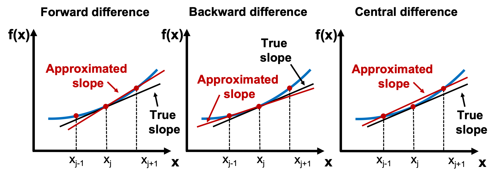
Because of its superior accuracy for a given step size $h$ , the central difference method is often the preferred choice for numerical differentiation. The following reading provides a more formal summary of these formulas and the Taylor series analysis.

Finite Difference Approximating Derivatives

This text from the Python Numerical Methods site at UC Berkeley provides a concise reference for the finite difference formulas and their derivation.

Please read the first two parts of the document: The introductory section, up to the first figure, which defines the three formulas. The section "Finite Difference Approximating Derivatives with Taylor Series," which shows how Taylor series are used to derive the formulas and quantify their error. Pay close attention to why the central difference is O(h^2).

From Single Derivatives to Gradient Vectors

We now have a method to approximate the derivative of a single-variable function. To compute the gradient of a multi-variable function, $\nabla f$ , we simply apply this method to calculate each partial derivative separately.

For a two-variable function $f (x, y)$ , the gradient is $\nabla f = ⟨ \frac{\partial f}{\partial x}, \frac{\partial f}{\partial y} ⟩$ . We can approximate each component using the central difference formula:

To find $\frac{\partial f}{\partial x}$ , we hold $y$ constant and perturb $x$ by $\pm h$ : $\frac{\partial f}{\partial x} (x, y) \approx \frac{f ( x + h , y ) - f ( x - h , y )}{2 h}$
To find $\frac{\partial f}{\partial y}$ , we hold $x$ constant and perturb $y$ by $\pm h$ : $\frac{\partial f}{\partial y} (x, y) \approx \frac{f ( x , y + h ) - f ( x , y - h )}{2 h}$

The numerical gradient is then the vector of these approximations. This process extends to any number of dimensions. For a point in a 3D dose grid, you would compute the partial derivatives along the x, y, and z axes one by one to assemble the full 3D dose gradient vector.

This grid illustrates the points used for finite difference calculations in 2D. To compute the partial derivatives at point $(i, j)$, we use its neighbors. The x-derivative uses points $(i-1, j)$ and $(i+1, j)$, while the y-derivative uses points $(i, j-1)$ and $(i, j+1)$.

Implementing Numerical Gradients in Python

Now, let's translate this logic into code. Your experience with Python and NumPy will make this process feel very natural. We will implement a general function that can compute the gradient of any Python function that takes a NumPy array as input.

The following resource provides a complete, practical example. It defines a sample "loss function" (a concept we'll formalize in the next module) and then builds a compute_gradient_numerical function to find its gradient.

Python Practice: Computing Gradients - ApX Machine Learning

This tutorial walks through a complete implementation of a numerical gradient calculator and demonstrates its accuracy.

Please read the entire article, paying close attention to the following sections: "Numerical Approximation of Partial Derivatives" and "Example Function": Understand the goal and the function we'll be differentiating. "Implementing Numerical Gradient Calculation with NumPy": This is the most important part. Study the Python code for compute_gradient_numerical. Notice how it iterates through each dimension of the input point and applies the central difference formula to compute one partial derivative at a time. "Running this code will output:": Compare the numerical gradient to the analytical one. The extremely small error demonstrates the effectiveness of the central difference method. "Importance and Limitations": This section provides crucial context. Numerical gradients are a powerful tool for verification but are too slow for training large models, which is why we will later learn about more efficient methods like backpropagation and automatic differentiation.

The function compute_gradient_numerical is a powerful tool. You could, for instance, define a Python function dose(coords) that calculates a dose value at a given [x, y, z] coordinate based on a mathematical model (like a summation of Gaussian beams). You could then pass this dose function and a specific coordinate array to compute_gradient_numerical to find the direction and magnitude of the steepest dose change at that exact point. This directly translates the abstract concept of $\nabla D$ into a concrete, computable value.

Conclusion

In this lesson, you've moved from the theory of gradients to their practical implementation. You now have a concrete method for calculating the "direction of steepest ascent" for any function you can define in code.

Key Takeaways:

Derivatives can be approximated numerically using finite difference formulas.
The central difference formula is typically preferred due to its higher accuracy ( $O (h^{2})$ ) compared to forward or backward differences ( $O (h)$ ).
A numerical gradient is computed by applying a 1D finite difference formula for each partial derivative of a multivariable function.
We can write a general-purpose function in Python and NumPy to compute the gradient of any function at any given point.

While powerful and universal, numerical differentiation is computationally expensive. For a function with $N$ variables (e.g., a neural network with $N$ parameters), it requires $2 N$ function evaluations to compute the gradient. For millions of parameters, this is prohibitively slow. It also has numerical precision pitfalls.

This limitation provides the perfect motivation for what's to come. In the next module, we will dive into the fundamentals of linear algebra and optimization, starting with how data and models are represented as vectors and matrices. We will then learn about gradient descent, the core optimization algorithm that uses gradients to iteratively improve a model. Finally, in later modules, you'll see how deep learning frameworks like PyTorch use a technique called automatic differentiation to compute exact gradients far more efficiently than the numerical methods we've learned today.

Recommended resources

Approximating Derivatives: The Finite Difference Method

From Single Derivatives to Gradient Vectors

Implementing Numerical Gradients in Python

Conclusion