Hello! Welcome back to our journey in building a C++ ray tracer.
In the last lesson, we explored the "why" of importance sampling. We established that the noise in our images is due to variance and that we can reduce it by sampling from a probability distribution that mimics the function we're trying to integrate. We learned the core formula for the Monte Carlo estimator with importance sampling:
where we draw samples from our new, "smarter" probability density function (PDF), .
Today, we move from theory to practice. Our goal is to implement arguably the single most important variance reduction technique in path tracing: sampling emissive objects directly. This technique is often called Next Event Estimation (NEE) and is fundamental to production renderers like Arnold and Karma. By the end of this lesson, you will have implemented a system that dramatically reduces noise by intelligently sending rays toward light sources.
Let's look at our target. This is a render of the Cornell Box with our current path tracer using 1000 samples per pixel.
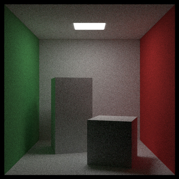
The graininess you see is variance. Our goal today is to attack that variance head-on.
1. The Problem: Finding the Needle in a Haystack
Why does our current renderer struggle so much with a simple scene like this? It comes down to probability. Our material's scattering function generates rays in random directions over the hemisphere. If the light source is small, the probability of a random ray happening to hit it is extremely low.
When a ray does hit the light, it returns a very bright color. When it misses, it returns a dark color (or black, if there are no other light bounces). The average of a few very bright samples and many dark samples results in a high-variance, noisy estimate.
To build a strong intuition for this problem and its solution, let's watch a video segment that explains it clearly.
TU Wien Rendering #25 - Path Tracing, Next Event Estimation
This lecture from TU Wien, 'Path Tracing, Next Event Estimation', clearly explains why naive path tracing struggles with small light sources and introduces the core idea of Next Event Estimation.
Please watch from 04:12 to 09:59. Focus on the explanation for why small light sources lead to slow convergence and how 'connecting the point to the light source' solves this.
As the video explains, the solution is to change our strategy. Instead of hoping a scattered ray finds a light, we will explicitly try to connect our shaded point to the light at every bounce. This means we will be generating two types of rays:
- A ray sampled from the material's BSDF (what we do now).
- A "shadow ray" aimed directly at a light source.
This is a form of importance sampling because we are choosing to sample directions we know are "important"—those pointing to lights. But to do this without introducing bias and making the image incorrectly bright, we need to derive the correct PDF for this new strategy.
2. Deriving the PDF for Direct Light Sampling
To use our importance sampling estimator, , we need to calculate —the probability density of generating a ray in a specific direction that points to a light.
Let's walk through the derivation, which you can also find in the Ray Tracing: The Rest of Your Life book.
Ray Tracing: The Rest of Your Life
This section of the book derives the mathematical formula for the PDF of sampling a light source. Understanding this is key to implementing importance sampling correctly.
Please read the subsection titled 'Getting the PDF of a Light'. The diagram and the derivation show how we convert a PDF over a surface area into a PDF over a solid angle.
Let's break down the logic:
-
Our strategy is to pick a random point, , uniformly on the surface of the light. If the light has a surface area of , the PDF of picking any specific point on that surface is constant: .
-
However, our rendering equation integrates over solid angle, not area. So, we need to find the PDF for sampling a direction, , from our shading point, , towards the light. Let's call this .
-
There's a geometric relationship between a small patch of area on the light and the solid angle that it covers from point :
Here, is the angle between the light's surface normal at and the vector from to . is the squared distance. -
The probability of choosing a direction within must be the same as choosing a point within . Therefore:
-
Now we substitute and solve for our desired PDF, :
This is our crucial formula. When we generate a ray by picking a point on a light, its probability density is the squared distance to that point, divided by the light's area and the cosine of the angle at the light's surface.
3. Combining Strategies with a Mixture PDF
We now have two distinct sampling strategies:
- BSDF Sampling: Using the material's properties (e.g., cosine-weighted sampling for diffuse surfaces).
- Light Sampling: Picking a point on a light source.
Which one is better? It depends!
- For a diffuse surface lit by a small, bright light, light sampling is far more effective.
- For a mirror reflecting a large area light (like a sky), BSDF sampling (which for a mirror is just a single reflection ray) is perfect, and light sampling would be wasteful.
Since no single strategy is always best, we'll combine them. We'll generate a new direction by randomly choosing between the two strategies. This is accomplished using a mixture PDF.
A mixture PDF is a weighted average of two or more PDFs. For our case, we'll use a 50/50 mix:
Here's how it works in practice:
- To generate a direction: We flip a coin (i.e., generate a random number). If it's less than 0.5, we generate a direction using BSDF sampling. Otherwise, we use light sampling.
- To evaluate the PDF value for a given direction: This is the subtle part. For any given direction, we must calculate the full mixture probability. We calculate the probability that either strategy could have produced that direction and add them up, weighted. So,
pdf_value = 0.5 * p_bsdf(dir) + 0.5 * p_light(dir).
The implementation of this is very clean using a mixture_pdf class.
Ray Tracing: The Rest of Your Life
The book now introduces the mixture_pdf class, which is the practical tool for combining our two sampling strategies.
Please read the subsection 'The Mixture PDF Class'. Pay close attention to the implementation of the value and generate methods, as they embody the logic we just discussed.
Test your understanding!
In our mixture PDF, why can't we just use the PDF of the strategy we chose to generate the ray? For example, if we chose light sampling to generate a ray, why is it incorrect to just say pdf_value = p_light(direction)?
Show answer
Because the other strategy (BSDF sampling) might also have been able to generate that same direction. For a diffuse surface, there is a non-zero probability of a cosine-sampled ray happening to point towards the light.
The total probability density for a direction is the sum of the weighted densities of all possible ways it could have been generated. If we only use the PDF of the chosen strategy, we are underestimating the true probability density for that direction. This would cause us to divide by a smaller number, incorrectly over-weighting the sample and introducing bias, resulting in an overly bright image. The full mixture PDF accounts for all paths, ensuring the estimate remains unbiased.
4. Implementation in the ray_color Loop
With the machinery of PDFs for lights and mixtures in place, we can finally update our main ray_color function. The logic will be more sophisticated, but the core idea is to replace our single scattered ray with one drawn from our new, powerful mixture distribution.
The implementation involves a few key changes, which are best understood by seeing them in context. I recommend reading through these sections from the book, which refactor the material class and the ray_color function to handle this new logic.
Ray Tracing: The Rest of Your Life
These sections show the final C++ implementation, tying everything together. They introduce a scatter_record to pass PDF information around and update ray_color to use the mixture PDF.
Please read the sections 'Cleaning Up PDF Management' and 'Adding PDF Functions to Hittable Lists'. You don't need to memorize every line of code, but trace the flow of logic in the ray_color function.
Let's summarize the new ray_color logic for a diffuse surface hit:
- Check for Emission: First, check if the surface we hit is itself emissive. If so, add its emitted light. This accounts for paths that terminate on a light source.
- Handle Speculars: If the material is purely specular (like a perfect mirror or glass), we skip all the PDF logic and just generate a single reflection/refraction ray. Importance sampling a delta function (like a perfect reflection) is easy—you just sample that one direction!
- Create Mixture PDF: For non-specular materials, create the two component PDFs:
light_pdf: Points to the light sources in the scene. Thehittable_listof lights now has methods to help with this.bsdf_pdf: Represents the material's scattering (e.g., acosine_pdf).- Combine them in a
mixture_pdf.
- Sample and Evaluate:
- Generate a new scattered ray by calling
mixture_pdf.generate(). - Calculate the PDF value for this new ray's direction with
pdf_value = mixture_pdf.value().
- Generate a new scattered ray by calling
- Calculate Contribution: Recursively call
ray_colorwith the new ray. The contribution from this scattered ray is then calculated using our master formula:
attenuation: The material's color (e.g., albedo).scattering_pdf: The value of the BSDF itself, representing in the rendering equation.pdf_value: The PDF of our mixture importance sampling strategy.
This final expression is the heart of a path tracer. The scattering_pdf / pdf_value term is the "MIS weight" that correctly balances the contribution of a sample based on how it was generated versus its physical properties.
When you run your code with these changes, the noisy image from the start of the lesson will be replaced by a much cleaner one, converging dramatically faster. This is the power of directing your samples to where the light is.
Conclusion
You have just implemented the core of a modern path tracing algorithm. By explicitly sampling light sources and robustly combining that strategy with BSDF sampling, you've taken a massive leap in rendering efficiency and quality.
Key Takeaways:
- Naive path tracing is noisy and inefficient for scenes with small lights because the probability of randomly hitting a light is very low.
- We solve this with Next Event Estimation (NEE), a form of importance sampling where we explicitly generate rays toward light sources.
- The PDF for sampling a light's surface is derived from solid angle-to-area conversion: .
- A mixture PDF provides a robust way to combine light sampling and BSDF sampling, allowing the renderer to efficiently handle a wide variety of materials and lighting conditions.
- The final Monte Carlo estimator weights the contribution of each sample by the ratio of the physical scattering distribution (
scattering_pdf) to the sampling distribution (pdf_value).
Next Steps
We are at the pinnacle of our ray tracer's development. We've implemented features that are conceptually identical to those in professional renderers. In our final lesson, we will step back and analyze what we've built. We'll compare our path tracer's architecture and techniques to those used in production renderers like Arnold and Karma, discussing what's needed to take a renderer like ours to the next level for feature film production.