The Rendering Equation: Foundation of Realistic Image Synthesis

1. Introducing the Rendering Equation

At its heart, the rendering equation is a mathematical statement that describes the "equilibrium" of light in a scene. It defines how much light, or more formally, radiance, leaves any given point on a surface in any given direction.

The core principle is elegantly simple:
Outgoing Light = Emitted Light + Reflected Light

A surface can generate its own light (if it's a light source), and it can reflect light that arrives from its surroundings. The rendering equation captures this with mathematical precision.

To get a quick and clear overview of its components, please watch this introductory video from NVIDIA.

Now, let's look at the equation itself and dissect it piece by piece.

A formal representation of the rendering equation, detailing each component. This equation is the cornerstone of physically-based rendering.

The equation is written as:
$L_o(x,{\vec{\omega }}_o)=L_e(x,{\vec{\omega }}_o)+{\int }_{\Omega }{f}_r(x,{\vec{\omega }}_i,{\vec{\omega }}_o)L_i(x,{\vec{\omega }}_i)(\vec{n}\cdot {\vec{\omega }}_i)d{\vec{\omega }}_i$

This might look intimidating, but it maps directly to our simple principle. Let's break it down using the excellent explanation from the "Introduction to the Rendering Equation" article.

Here is a summary of the key terms:

• $L_o(x,{\vec{\omega }}_o)$: This is the outgoing radiance from point $x$ in the direction ${\vec{\omega }}_o$. This is the quantity we want to compute—the "color" of a surface point as seen from a particular direction.

• $L_e(x,{\vec{\omega }}_o)$: This is the emitted radiance. It's the light that the surface at point $x$ emits on its own. For most objects, this is zero. For the light sources you created in the last lesson, this is a non-zero color.

• ${\int }_{\Omega }\dots d{\vec{\omega }}_i$: This integral represents the reflected radiance. It sums up all the light that comes in from every possible direction over the hemisphere $\Omega$ above point $x$, and determines how it reflects towards the viewer.

The three terms inside the integral are the heart of the light reflection model:

1. $f_r(x,{\vec{\omega }}_i,{\vec{\omega }}_o)$: The Bidirectional Reflectance Distribution Function (BRDF).
   • This function is the material. It defines how a surface reflects light. It answers the question: "For light coming in from direction ${\vec{\omega }}_i$, what fraction is scattered out in direction ${\vec{\omega }}_o$?"
   • A diffuse (Lambertian) material has a BRDF that scatters light equally in all directions. A metallic material has a BRDF that scatters light in a narrow, mirror-like lobe. Your scatter function in the material class is an implementation of this concept.

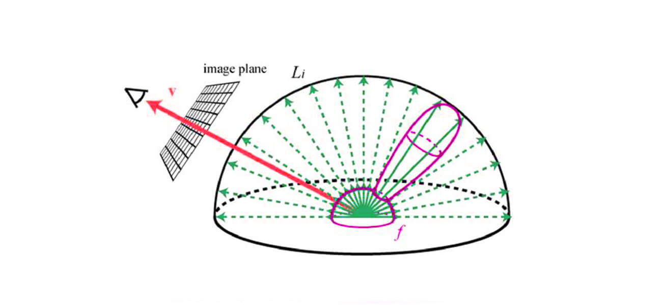
*This diagram visualizes the core of the rendering equation's integral: light arriving from many incoming directions ($L_i$) is reflected by the surface's material properties (the BRDF, $f$) toward the camera's view direction ($v$).*

2. $L_i(x,{\vec{\omega }}_i)$: The incoming radiance.
- This represents the light arriving at point $x$ from direction ${\vec{\omega }}_i$. This is the crucial part that makes the equation recursive. The light arriving at our point $x$ is simply the outgoing light from some other point in the scene that lies in the direction ${\vec{\omega }}_i$. To find $L_i$, we must solve the rendering equation for that other point! This recursive nature is exactly why we use ray tracing to solve it.

3. $(\vec{n}\cdot {\vec{\omega }}_i)$: The cosine term.
   • This term, also written as $\cos {\theta }_i$, accounts for the angle at which incoming light strikes the surface. As explained in the geometrian.com article, light arriving at a shallow or grazing angle is spread over a larger surface area, so its contribution to the outgoing radiance is diminished. This is Lambert's cosine law, the same principle that makes the poles of the Earth colder than the equator.

2. Connecting the Equation to Your Code

The abstract math of the rendering equation directly maps to the ray_color function you've already written. Let's make that connection explicit:

• $L_o(x,{\vec{\omega }}_o)$ is the final color value that your ray_color function returns.
• $L_e(x,{\vec{\omega }}_o)$ is the emitted color you get from rec.mat_ptr->emitted(...).
• ${\int }_{\Omega }{f}_r(...)L_i(...)(\vec{n}\cdot {\vec{\omega }}_i)d{\vec{\omega }}_i$ is what you are approximating with the line attenuation * ray_color(scattered, world, depth-1).

How is that one line of code an approximation of a complex integral?

• When you call your scatter function, it generates a single scattered ray direction. This is like picking just one ${\vec{\omega }}_i$ from the entire hemisphere $\Omega$.
• The attenuation color returned by scatter is a simplified combination of the BRDF $f_r$ and the cosine term $(\vec{n}\cdot {\vec{\omega }}_i)$. For a Lambertian material, the attenuation is constant, and the random scattering direction implicitly handles the cosine term.
• The recursive call ray_color(scattered, ...) is literally solving for $L_i$, the incoming light from that one chosen direction.

So, your path tracer is solving the rendering equation by sampling one light path at a time and accumulating the result. This is a Monte Carlo approach, which we'll formalize in the next lesson.

3. Global Illumination and Light Bounces

The rendering equation provides a powerful framework for thinking about light transport. One of the most elegant ways to view it is using operator notation, as shown in the presentation slides from TU Wien.

The equation $L_o=L_e+\int \dots$ can be written more compactly as:
$L=L_e+T(L)$

Here, $L$ represents the light field of the entire scene, $L_e$ is the emitted light, and $T$ is a "transport operator" that describes one bounce of light. It takes the existing light field $L$, propagates it through the scene, reflects it off surfaces, and gives you the result after one bounce.

By expanding this equation, we get a beautiful series:
$L=L_e+T(L_e)+T(T(L_e))+T(T(T(L_e)))+\dots$
$L=L_e+T^1{L}_e+T^2{L}_e+T^3{L}_e+\dots$

This reveals exactly what your path tracer is simulating:

• $L_e$: Light seen directly from a light source (0 bounces).
• $T^1{L}_e$: Light that has bounced once before reaching the eye (indirect illumination). This is what lights up the ceiling in a room with an upward-facing lamp.
• $T^2{L}_e$: Light that has bounced twice (secondary indirect illumination). This is responsible for subtle effects like color bleeding, where a red wall will cast a faint red tint on a nearby white wall.
• And so on for all subsequent bounces.

The sum of all these terms is called Global Illumination (GI). It's the "Holy Grail" of realistic rendering, and the rendering equation gives us the complete recipe for it.

The following video discusses this concept by splitting the rendering equation into practical components that renderers often compute separately.

As the video explains, many renderers (especially real-time ones, but also offline renderers for optimization) treat direct and indirect light differently. Direct lighting can sometimes be computed more efficiently, while the multi-bounce indirect lighting is often the most computationally expensive part of rendering, responsible for the richest and most subtle visual effects.

Conclusion

Today, we've pulled back the curtain on path tracing to reveal the solid mathematical foundation it's built upon. You've learned that your renderer is, in fact, a solver for a fundamental equation of light transport.

Key Takeaways:

• The Rendering Equation is the formal basis for physically-based rendering, stating that Outgoing Light = Emitted Light + Reflected Light.
• The reflected light component is an integral over the hemisphere that accounts for all incoming light, modulated by the material's BRDF and the cosine of the incidence angle.
• The equation is recursive in nature, as incoming light to one point is outgoing light from another. This is why ray tracing is such a natural fit for solving it.
• Your ray_color function is a practical implementation that approximates the equation by tracing one path of light at a time.
• Global Illumination is the complete solution to the equation, accounting for multiple bounces of light (direct and indirect), which are responsible for effects like soft shadows and color bleeding.

Next Steps

We've established that the rendering equation contains an integral and that your path tracer is approximating it by picking a random direction at each bounce. But is this approximation correct? How many samples do we need? And can we do better?

In the next lesson, we will formalize this process. You will learn how path tracing serves as a Monte Carlo method to solve the rendering equation. We'll explore the theory of Monte Carlo integration and see why our seemingly simple random-sampling approach converges to the physically correct solution.