Understanding Monte Carlo Noise

1. The Nature of a Random Estimate

At its heart, the Monte Carlo method uses randomness to estimate a deterministic value. Whether we're estimating the value of $\pi$ or the color of a pixel, the process is the same: take many random samples and average them. The "law of large numbers" guarantees that as we take more samples, our average will get closer to the true value. But what happens when we have only a few samples? The estimate fluctuates.

To build a strong intuition for this, let's watch a video that illustrates the core idea of Monte Carlo simulation.

The key takeaway is that with a small number of samples, your estimate can be far from the true value simply due to bad luck. As you add more samples, the influence of any single "unlucky" sample is diminished, and the average converges.

2. From Fluctuation to Visual Noise

The fluctuation you saw in the Pi estimation is exactly what causes noise in your rendered images. Each pixel in your final image is an independent Monte Carlo estimation of the light arriving from the scene.

• The integral: The rendering equation's integral over the hemisphere.
• The true value: The real, correct color of that pixel.
• The samples: Each full path traced from the camera for that pixel.
• The estimate: The average color of all paths for that pixel.

When you use a low number of samples per pixel (SPP), the estimate for one pixel might be a bit too high (a lucky path hit a bright spot), while the estimate for its neighbor might be too low. This pixel-to-pixel difference in estimation error is what our eyes perceive as noise or grain.

Let's see this in action. The same video you just watched has a perfect demonstration.

To reinforce this, here is a classic image from rendering literature that makes the trade-off between sample count, noise, and render time crystal clear.

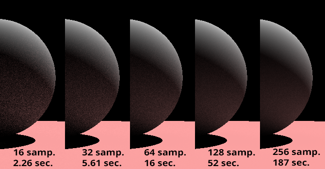
This relationship between sample count and noise is fundamental. To get a more formal handle on it, let's read a short explanation.

The article highlights a crucial point: to reduce noise by half, you need four times as many samples. This isn't just an observation; it's a consequence of the mathematics behind the noise.

3. The Mathematics of Noise: Variance

The term for this statistical fluctuation is variance. Variance measures how spread out a set of random values are from their average. In path tracing, high variance means that individual path samples for a pixel can have wildly different color values, leading to a noisy final average. Low variance means the samples are all fairly similar, leading to a clean, stable average.

The previous lesson introduced this concept, but let's look at the math more closely. The standard deviation, $\sigma$, which is the square root of the variance, is what we perceive as noise. For a Monte Carlo estimator, it has a very specific form.

The most important equation from that section is:
$\sigma =\frac{1}{\sqrt{N}}\sqrt{\mathbb{V}ar\left[\frac{f(X_1)}{p(X_1)}\right]}$
Let's break this down:

• $\sigma$ is the standard deviation—the "amount" of noise we see.
• $N$ is the number of samples (paths per pixel).
• $f(X)$ is the function we are integrating (the terms inside the rendering equation integral).
• $p(X)$ is the probability density function (PDF) of our sampling strategy.

This formula mathematically confirms what we've observed:

1. The noise $\sigma$ is proportional to $1/\sqrt{N}$. This is why you must quadruple the samples ($N$) to halve the noise ($\sigma$).
2. The noise also depends on the variance of the function being sampled. The term $\mathbb{V}ar\left[\frac{f(X)}{p(X)}\right]$ is crucial. If this term is large, the image will be noisy even with many samples.

4. What Causes High Variance?

So, when is the variance term $\mathbb{V}ar\left[\frac{f(X)}{p(X)}\right]$ large? It happens when the values of $\frac{f(X)}{p(X)}$ fluctuate wildly. This occurs when our sampling strategy gives us a low probability ($p(X)$ is small) of hitting a sample with a very high contribution ($f(X)$ is large).

The classic example in rendering is a small, bright light source in an otherwise dark scene.

• Our current uniform sampling strategy sends rays in all directions equally. The probability of a ray randomly hitting the small light source is very low.
• Most rays will hit a dark wall, contributing almost no light ($f(X)\approx 0$).
• Once in a while, a lucky ray will hit the light source, contributing a massive amount of energy ($f(X)$ is huge).

The average is pulled around by these rare, super-bright samples. This creates high variance, which manifests as "fireflies"—individual pixels that are unnaturally bright.

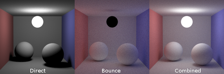
Indirect lighting (light that has bounced at least once) is particularly prone to this. The direct light from a source can often be calculated quite accurately, but the bounced light relies entirely on the Monte Carlo estimation of where that light goes next.

Conclusion

In this lesson, we have formally connected the dots between the random sampling process of path tracing and the resulting visual noise in the final image.

Key Takeaways:

• Visual noise in a path-traced image is a direct manifestation of statistical variance in the Monte Carlo estimation of pixel color.
• Variance arises because we are averaging the results of random paths, and the light contribution from each path can differ significantly.
• Noise decreases proportionally to the square root of the number of samples ($1/\sqrt{N}$), meaning we must quadruple the samples to halve the noise.
• High variance occurs when our sampling strategy has a low probability of finding high-energy contributions, such as small, bright light sources. This results in "fireflies" and excessive grain.

Next Steps

We have now thoroughly diagnosed the problem: noise is variance. Brute-forcing more samples is a solution, but it's incredibly inefficient. The formula for variance, $\mathbb{V}ar\left[\frac{f(X)}{p(X)}\right]$, points to a much more elegant solution. Instead of just increasing $N$, what if we could reduce the variance term itself?

In our next lesson, we will begin our exploration of importance sampling. You will learn how to design "smarter" sampling strategies ($p(X)$) that are more likely to find the important, high-energy paths of light. This is the key to dramatically reducing noise and is a cornerstone of all modern production renderers.