Fast Ray-AABB Intersection

1. The "Slab" Method Revisited

Let's quickly recap the core algorithm we're implementing: the slab test. An AABB is the intersection of three pairs of axis-aligned planes (slabs). A ray hits the box if, and only if, the segments of the ray inside each of the three slabs overlap.

Each slab defines an interval [t_min, t_max] along the ray. We find the overall intersection interval by taking the maximum of all t_min values and the minimum of all t_max values. An intersection occurs if this final interval is valid (i.e., t_final_min < t_final_max).

This image provides an excellent visual breakdown of the process in 2D.

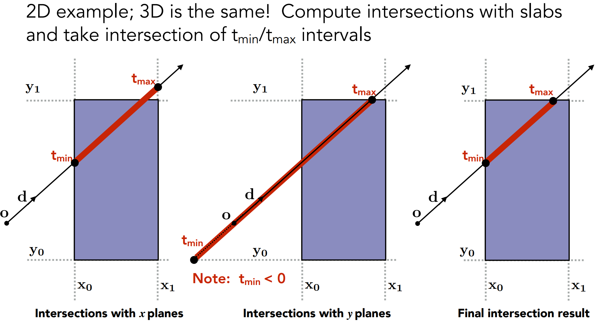
The key insight is that we can process each axis independently and accumulate the result.

2. A Robust and Fast Implementation

A naive implementation of the slab method can be slow and prone to numerical errors. A production-quality function must be both fast and robust. Let's explore the key components of such an implementation.

The Core Algorithm

First, let's review the fundamental logic and the mathematical derivation. Both of the following resources provide excellent explanations of the slab test, starting from the ray equation and deriving the intersection logic.

Optimization Strategy 1: The Curse of Division

In the formula t = (plane_pos - ray_origin) / ray_direction, the division is computationally more expensive than multiplication. Since we will call this intersection function billions of times when rendering a complex scene, every saved instruction matters.

The standard optimization is to pre-calculate the inverse of the ray's direction components (1/d.x, 1/d.y, 1/d.z) once when the ray is created. Then, the intersection calculation becomes a much faster multiplication: t = (plane_pos - ray_origin) * inv_ray_direction.

Optimization Strategy 2: Handling Ray Direction

What happens if the ray travels in a negative direction along an axis (e.g., d.x < 0)? The t value for the min plane (x_0) will be larger than the t for the max plane (x_1). Our computed t-interval will be "reversed," like [7, 3].

There are two elegant ways to handle this without expensive branching:

1. The min/max approach: As seen in Ray Tracing: The Next Week, you can compute both t0 and t1 and then use min() and max() to sort them into the correct [t_min, t_max] interval. This is conceptually simple but involves an extra comparison.
2. The swap approach: Compute t_min and t_max assuming a positive direction. If t_min > t_max, swap them.
3. The sign-precomputation approach: This is a very slick optimization. Before any tests, you determine the sign of each component of the ray's direction. You can then use this sign to fetch the correct box boundaries (min or max) directly, eliminating the need for a swap.

The resource from Scratchapixel provides a fantastic, detailed walkthrough that culminates in this highly optimized version.

3. Final Implementation and Robustness

Now let's look at the full C++ implementation from Ray Tracing: The Next Week, which we saw in the last lesson. This time, analyze it through the lens of performance and robustness.

A final point on robustness: what if an object is perfectly flat, like a quad aligned with the XY plane? Its AABB would have zero thickness in the Z dimension. This can cause floating-point precision issues for rays that are nearly parallel to the object. A common solution is to ensure every AABB has a small, non-zero thickness on all axes by "padding" it slightly. This is discussed in section 5 of the AABB chapter in Ray Tracing: The Next Week (resource LINK), which you can review if you're interested in making your implementation even more robust.

4. The Bigger Picture: A Glimpse into BVH Traversal

Why this obsession with speed? Because this intersection test is the most frequently called function in the entire BVH acceleration process. For each ray, the renderer will traverse the BVH tree, calling aabb::hit() at each node.

In the video below, the presenter implements a BVH and discovers an important optimization. The aabb::hit function can be made even more useful if, instead of returning a simple true/false, it also returns the distance t to the intersection point. This allows the traversal algorithm to intelligently skip entire branches of the tree that are further away than an already-found intersection.

We won't implement this distance-based optimization just yet, but it's a fantastic example of how a well-designed, low-level function enables high-level algorithmic improvements.

Conclusion

In this lesson, we took a magnifying glass to the ray-AABB intersection test, moving from a basic working function to a deep understanding of how to make it fast and robust.

Key Takeaways:

• The Slab Test is King: It's an elegant, component-wise algorithm for ray-AABB intersection.
• Optimization is Non-Negotiable: For a function this critical, you must optimize. Pre-calculating the inverse ray direction is the most important first step.
• Handle All Directions: A robust implementation must correctly handle rays traveling in negative directions, either through logic (swaps, if/else) or clever data structures (sign array).
• Floating-Point is Tricky: Understanding how IEEE 754 handles infinities helps write simpler code for edge cases like parallel rays. Padding boxes ensures robustness for flat objects.
• Informing Higher-Level Algorithms: The design of this low-level function (e.g., returning t vs. a bool) has a direct impact on the efficiency of the larger BVH traversal algorithm.

Next Steps

We now have our razor-sharp tool: a fast, robust aabb::hit() function. In the next lesson, we will finally put it to work. We'll use it as the core component to construct a Bounding Volume Hierarchy, recursively subdividing our scene geometry and building the tree structure that will accelerate our renders from minutes to seconds.