Iterative Bayesian Updating for Style Refinement

Introduction

In our last lesson, we established a framework for evaluating a single lingerie screening step, calculating the Positive Predictive Value (PPV) and False Positive Rate (FPR) to understand the effectiveness of our initial selection process. We saw that the PPV is simply the posterior probability, $P (Style is a Star ∣ Selected)$ , after considering one piece of evidence. Today, we will take this concept a step further by exploring what happens as we gather more evidence during the fitting and testing process.

This lesson focuses on the dynamic and powerful technique of iterative Bayesian updating. You will learn how to use the posterior probability from one observation as the prior belief for the next, allowing you to sequentially refine your assessment of a lingerie style's potential. This mirrors the real-world process of a fitting room, where your confidence in a piece evolves with each pose, lighting change, and accessory pairing.

The Logic of Sequential Updating

Bayesian inference is not a static, one-time calculation. It is a continuous learning process. The posterior probability you calculate after observing one piece of evidence represents your new, updated state of belief. If you then acquire another piece of evidence, this posterior becomes the prior for your next calculation.

This creates a powerful iterative loop:

Prior_{1} Evidence_{1} Posterior_{1} \to Prior_{2} Evidence_{2} Posterior_{2} \to \dots

This sequential process is analogous to updating the state of a system in a discrete-time stochastic process. Each new observation—a successful test shot, a positive comment from the model—moves you to a new belief state, progressively honing your estimate of the style's true potential.

The Beta-Binomial Model: Your Toolkit for Fitting Room Data

Given your background in statistics, the most elegant framework for modeling this iterative process is the Beta-Binomial conjugate model. It's perfectly suited for your goal of estimating the "star quality" of a lingerie piece.

Let's define the components:

The Parameter of Interest ( $π$ ): Let $π$ be the true, unknown probability that a specific lingerie piece is a "winner" for this photoshoot. It represents its inherent appeal or "star quality," a value between 0 and 1. Our goal is to estimate $π$ .
The Prior (Beta Distribution): Our initial belief about $π$ can be modeled using a Beta distribution, written as $Beta (α, β)$ .
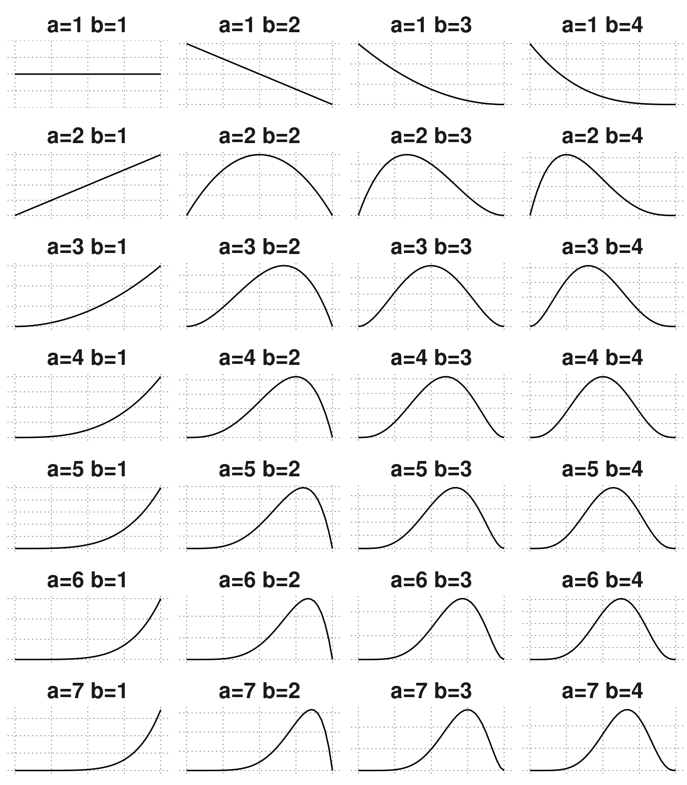
- The parameters $α$ and $β$ can be intuitively thought of as counts of prior "successes" and "failures." For example, if past experience with similar styles suggests they work about half the time, but you're not very certain, you might start with a $Beta (2, 2)$ prior. A $Beta (1, 1)$ prior is a uniform distribution, representing complete uncertainty—any value of $π$ is equally likely.
- The image below shows how different choices of a ( $α$ ) and b ( $β$ ) create a wide variety of belief shapes, from optimistic (a > b) to skeptical (b > a) to uncertain (low a and b).

A grid showing various shapes of the Beta probability density function for different shape parameters, `a` and `b`. This illustrates the flexibility of the Beta distribution in representing prior beliefs.

The Likelihood (Binomial Distribution): New evidence from a fitting session can be modeled as a series of Bernoulli trials, which collectively follow a Binomial distribution. For example, you take $n$ test shots and observe $k$ "successful" shots that perfectly capture the desired look. The likelihood of observing this outcome, given a certain "star quality" $π$ , is governed by the Binomial probability mass function.
The Posterior (Beta Distribution): The power of using a Beta distribution for the prior and a Binomial distribution for the likelihood is that they are a conjugate pair. This means the posterior distribution is also a Beta distribution. The update rule is incredibly simple:

If your prior is $Beta (α, β)$ and you observe $k$ successes in $n$ trials, your new posterior distribution for $π$ is:
$Posterior = Beta (α_{prior} + k, β_{prior} + n - k)$

You simply add the new successes to $α$ and the new failures to $β$ . This provides a computationally trivial way to update your beliefs without recalculating Bayes' theorem from scratch each time.

Visualizing the Iterative Process

The following grid of plots masterfully illustrates this sequential updating process. Each row represents a different starting prior belief, and each column shows the belief updating as more data is collected.

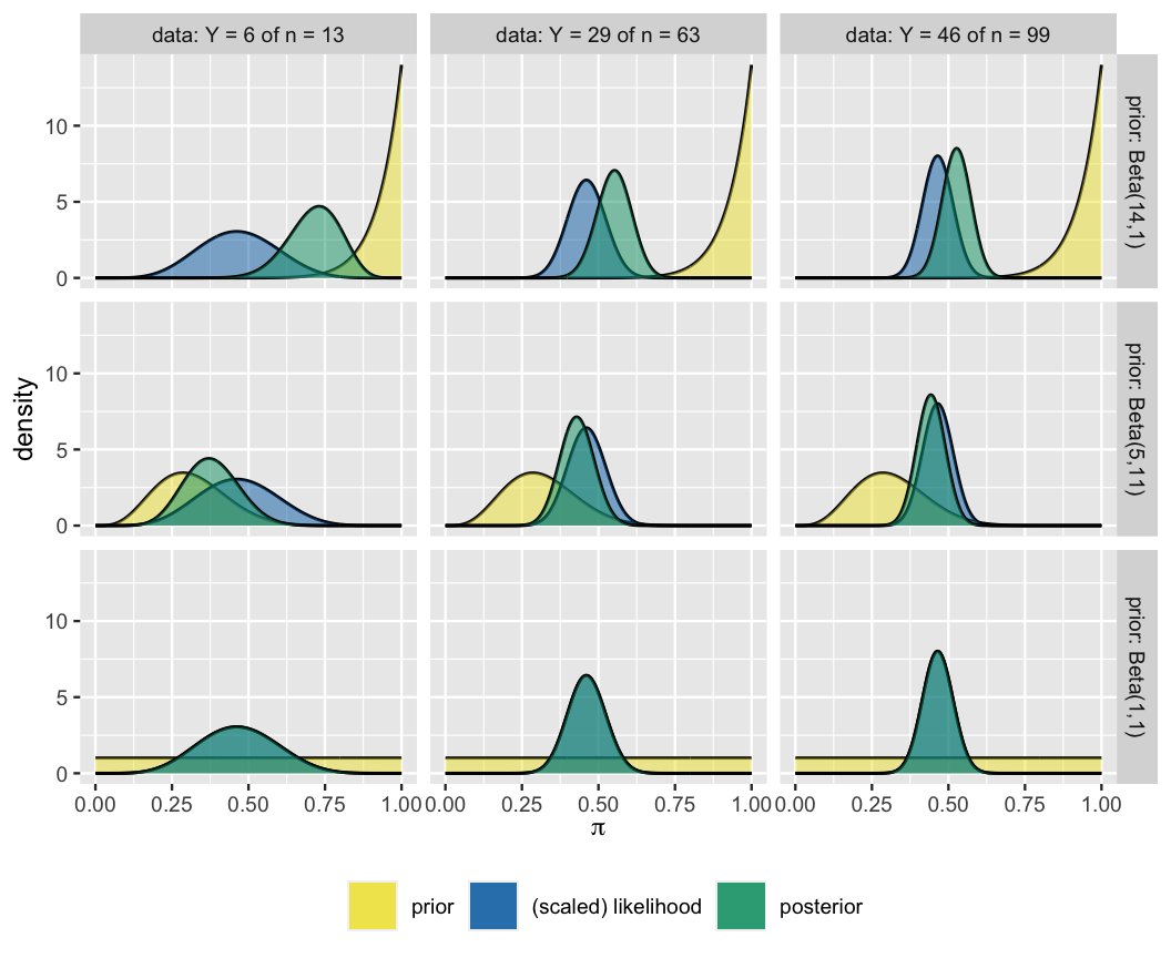
A grid of plots demonstrating Bayesian updating. Each row starts with a different prior (yellow). As data comes in (n=13, n=63, n=99), the likelihood (blue) and the resulting posterior (green) are shown. The posterior is a compromise between the prior and the likelihood.

Let's trace the middle row as an example of an iterative fitting session for a promising style:

Prior Belief: We start with a Beta(5.1, 1) prior (the yellow curve in the middle-left plot). This is an optimistic belief; we think this style has a high probability of being a winner, perhaps because it comes from a trusted designer. The peak of our belief is high.
First Fitting (Evidence 1): We conduct an initial tryout with $n = 13$ poses and find that $Y = 6$ are successful. The data itself suggests a success rate of 6/13 ≈ 46%. This evidence is represented by the blue "likelihood" curve. The resulting posterior belief (the green curve) is a compromise. It has shifted our initial optimism to the left, moderated by the actual data. This Beta(5.1+6, 1+13-6) = Beta(11.1, 8) distribution is our new, updated belief.
Second Fitting (Evidence 2): Now, we use that posterior as our new prior. We conduct a larger set of test shots, bringing the total to $n = 63$ with $Y = 29$ total successes. The new evidence provides a narrower likelihood curve (middle plot). Our belief updates again.
Final Assessment (Evidence 3): After a full session with $n = 99$ data points (e.g., shots, poses, angles) and $Y = 46$ successes, our final posterior (middle-right plot) is even more precise.

Notice two critical things as you move from left to right:

The posterior distribution becomes narrower (less variance), reflecting our growing certainty as we collect more data.
The influence of the initial prior diminishes. The final posterior is dominated by the accumulated evidence (the likelihood).

This is the essence of data-driven decision-making in a Bayesian framework.

Numerical Exercise: Iterative Evaluation of a Lace Balconette

Let's apply this to a concrete fitting room scenario. You are evaluating a new "Delicate Lace Balconette" bra. You have no prior experience with this specific style, so you approach it with an open mind.

Your Task:

Initial Prior: You decide to use an uninformative prior to represent your initial uncertainty. What Beta distribution should you choose?
First Fitting: The model tries the bra. In a series of 5 test poses, the photographer gives a "thumbs up" to 3 of them. What is your new posterior distribution for $π$ , the "star quality" of this bra?
Second Fitting: You like the initial results and decide to test the bra with a more complex lighting setup. This time, in 10 shots, you get 8 "thumbs up." Using your posterior from the first fitting as your new prior, calculate the final posterior distribution after this second round of evidence.
Interpretation: Compare your initial prior with your final posterior. How has your belief about the bra's potential evolved? Calculate the mode (the peak of the distribution) for your final belief. The mode of a $Beta (α, β)$ distribution is $(α - 1) / (α + β - 2)$ .

Solution

Initial Prior: An uninformative prior, representing complete uncertainty, is the Uniform distribution, which is a special case of the Beta distribution: $Beta(1, 1)$ . Here, $α = 1$ and $β = 1$ .
First Fitting Update:
- Prior: $Beta (1, 1)$
- Evidence: $k = 3$ successes in $n = 5$ trials. This means there were $n - k = 2$ failures.
- Posterior: $Beta (1 + 3, 1 + 2) = Beta(4, 3)$ .
  Our belief has shifted from uniform to one that peaks around a success probability of $π \approx 0.6$ .
Second Fitting Update:
- New Prior: $Beta (4, 3)$
- New Evidence: $k = 8$ successes in $n = 10$ trials. This means there were $n - k = 2$ failures.
- Final Posterior: $Beta (4 + 8, 3 + 2) = Beta(12, 5)$ .
Interpretation:
We started with a $Beta (1, 1)$ distribution, where any "star quality" $π$ from 0 to 1 was equally plausible. After two rounds of fittings, our belief is now described by a $Beta (12, 5)$ distribution. This distribution is sharply peaked, indicating a much higher degree of certainty. Our belief has evolved from "I have no idea" to "I am quite confident this is a strong piece."

The mode of our final posterior belief is:
$Mode = \frac{α - 1}{α + β - 2} = \frac{12 - 1}{12 + 5 - 2} = \frac{11}{15} \approx 0.733$
Our single most likely estimate for this bra's "star quality" is now approximately 73.3%.

Conclusion

In this lesson, we moved from static evaluation to a dynamic, iterative process of belief updating. You learned how to sequentially refine your assessment of a lingerie style's potential as new evidence becomes available from fittings and test shots.

Key Takeaways:

Bayesian inference is a process of sequential learning where the posterior from one step becomes the prior for the next.
The Beta-Binomial conjugate model is an exceptionally practical tool for this. Your belief about a style's "star quality" ( $π$ ) is represented by a Beta distribution.
Updating your belief is as simple as adding new successes to the $α$ parameter and new failures to the $β$ parameter of your Beta distribution.
As more data accumulates, your posterior belief becomes more precise, and the influence of your initial, subjective prior diminishes.

You now have the core mechanism for dynamically evaluating and comparing styles. In our next lesson, we will synthesize the concepts from this module in a final numerical problem. You will be given prior beliefs for three competing lingerie styles and a single set of new evidence. Your task will be to perform the iterative update for each one and use their final posterior probabilities to rank them and make a selection.