Predicting Photoshoot-Worthy Lingerie with Naive Bayes

Welcome to the first lesson in our module on classification models. In our previous module, we delved deep into the world of causal inference, focusing on answering "why" a certain lingerie style performs well by using tools like DAGs and the adjustment formula. Now, we pivot from explanation to prediction. Our goal is no longer to estimate a causal effect but to build models that can accurately predict an outcome, such as whether a new design will be a 'top pick' for a photoshoot.

This lesson introduces our first classification algorithm: the Naive Bayes classifier. Given your background in Bayesian Decision Theory, the foundational theorem will be very familiar. Our focus will be on its practical application and the crucial—and simplifying—"naive" assumption that makes it so efficient. We will learn how to apply this model to predict if a new lingerie piece is 'photoshoot-worthy' based on its categorical features like fabric, color, and type, directly addressing this lesson's learning outcome.

Bayes' Theorem in a Nutshell

At the heart of the Naive Bayes classifier is Bayes' theorem, which provides a way to update our beliefs in light of new evidence. In a classification context, we want to find the probability of a class (e.g., 'photoshoot-worthy') given a set of features (e.g., fabric, color).

The theorem is expressed as:

P (Class ∣ Features) = \frac{P ( Features ∣ Class ) \times P ( Class )}{P ( Features )}

Each term has a specific name and role, as illustrated below.

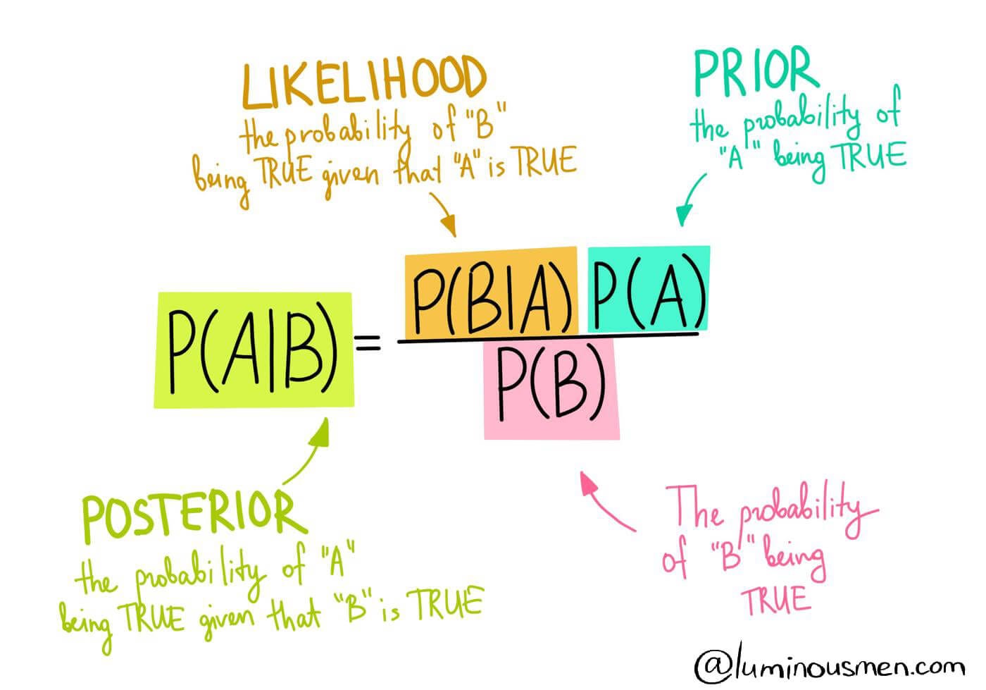
This diagram breaks down Bayes' Theorem into its four components: the Posterior probability, the Likelihood, the Prior probability, and the probability of the Evidence. In our context, 'A' is the class (e.g., Photoshoot-Worthy) and 'B' is the evidence or features (e.g., a red lace bralette).

Prior $P (Class)$ : Our initial belief about the probability of a class before seeing any features. For example, what percentage of all lingerie pieces in our collection are 'photoshoot-worthy'?
Likelihood $P (Features ∣ Class)$ : The probability of observing a certain set of features, given that a piece belongs to a specific class. For example, what is the probability of a piece being made of lace and colored red, given that it is 'photoshoot-worthy'?
Evidence $P (Features)$ : The overall probability of observing this set of features, across all classes.
Posterior $P (Class ∣ Features)$ : The updated probability of the class after observing the features. This is what we want to calculate.

The "Naive" Assumption: A Key Simplification

Calculating the likelihood $P (Features ∣ Class)$ directly is difficult because it requires us to know the joint probability of all features, which can be complex. The Naive Bayes classifier makes a powerful simplifying assumption: all features are conditionally independent of each other, given the class.

In our lingerie example, this means we assume that for a 'photoshoot-worthy' piece, its fabric tells us nothing about its color or type, and vice-versa. While this is rarely true in reality (certain fabrics might be more common for certain types, like lace for bralettes), this "naive" assumption allows us to break down the complex likelihood calculation into a simple product of individual probabilities.

The following resource provides the formal mathematical justification for this simplification.

1.9. Naive Bayes

This document introduces the core mathematics of Naive Bayes classifiers. Pay close attention to how Bayes' theorem is transformed by the conditional independence assumption.

Read the introductory section, from the start down to the classification rule. Note how the joint probability P(x_1, \dots, x_n \mid y) is simplified into the product \prod_{i=1}^{n} P(x_i \mid y).

With this assumption, our classification rule becomes: find the class $y$ that maximizes the product of the prior and the individual likelihoods.

y^= ar g y max P (y) i = 1 \prod n P (x_{i} ∣ y)

We can ignore the denominator $P (Features)$ because it's the same for all classes and thus doesn't affect which class has the highest posterior probability.

Classifying Lingerie with Categorical Naive Bayes

Our features—Fabric, Color, Type—are categorical. For this, we use a specific variant called Categorical Naive Bayes. This model estimates the likelihood $P (x_{i} ∣ y)$ for each feature category by simply counting frequencies in the training data.

To avoid issues with categories that don't appear in the training data for a certain class (which would result in a probability of zero, nullifying the entire product), we use a smoothing technique. The most common is Laplace smoothing (or Lidstone smoothing), where we add a small value $α$ (usually 1) to our counts.

The scikit-learn documentation explains this process clearly.

1.9. Naive Bayes

This section provides the exact formula for calculating probabilities for categorical features, including the smoothing parameter.

Focus on the subsection "Categorical Naive Bayes". The formula presented here is exactly what we will use in our numerical exercise. Understand what each term—N_{tic}, N_c, \alpha, and n_i—represents.

The core idea of using categorical features (like clothing items) to classify something (like music genre) is explored in the following paper. It uses a method analogous to what we are doing for lingerie.

[PDF] Automatic Classification of Artist Visual Aesthetics: Linking Fashion ...

This paper applies machine learning to classify music genres based on fashion. It's a great parallel to our task of classifying lingerie based on design attributes.

Read the section "Genre Classification". Notice how the authors treat clothing items as a "bag-of-words" and explicitly mention Naive Bayes as a suitable classifier for this type of data. This validates our approach of treating lingerie features as a collection of independent categorical attributes.

Your Turn: A Numerical Application

Now, let's apply this to a concrete problem. Your strong statistical background will be invaluable as you calculate the probabilities step-by-step.

Scenario:
You have a small training dataset of 15 lingerie pieces, each with three categorical features (Fabric, Color, Type) and a binary outcome (Photoshoot-Worthy: Yes/No).

Fabric	Color	Type	Photoshoot-Worthy
Lace	Black	Bralette	Yes
Satin	Red	Push-up	Yes
Lace	Black	Push-up	Yes
Cotton	Nude	Bralette	No
Satin	Black	Balconette	Yes
Lace	Red	Bralette	Yes
Cotton	Black	Bralette	No
Satin	Nude	Push-up	No
Lace	Nude	Balconette	Yes
Cotton	Red	Bralette	No
Lace	Black	Balconette	Yes
Satin	Red	Push-up	Yes
Cotton	Nude	Push-up	No
Lace	Red	Bralette	Yes
Satin	Black	Balconette	No

Your Task:
A new piece has arrived: a Red Lace Bralette. Your goal is to predict if it is 'Photoshoot-Worthy' using the Naive Bayes classifier. Use Laplace smoothing with $α = 1$ .

Calculate the Priors:
- $P (Worthy = Yes)$
- $P (Worthy = No)$
Calculate the Likelihoods:
For both Yes and No classes, calculate the conditional probabilities for the new piece's features: Fabric=Lace, Color=Red, Type=Bralette. Remember to use the smoothing formula:
$P (x_{i} = t ∣ y = c) = \frac{N _{t i c} + α}{N _{c} + α \cdot n _{i}}$
Where $N_{c}$ is the count of class $c$ , $N_{t i c}$ is the count of feature $t$ in class $c$ , and $n_{i}$ is the number of unique categories for that feature.
Calculate the Posteriors (Proportional):
- Calculate $P (Worthy = Yes) \times P (Lace|Yes) \times P (Red|Yes) \times P (Bralette|Yes)$ .
- Calculate $P (Worthy = No) \times P (Lace|No) \times P (Red|No) \times P (Bralette|No)$ .
Classify:
Which class has the higher score? Predict whether the Red Lace Bralette is 'Photoshoot-Worthy'.

Click for the step-by-step solution.

1. Calculate Priors
There are 15 total samples.

Count(Worthy = Yes) = 9
Count(Worthy = No) = 6
$P (Worthy = Yes) = \frac{9}{15} = 0.6$
$P (Worthy = No) = \frac{6}{15} = 0.4$

2. Calculate Likelihoods (with $α = 1$ )

First, let's count the number of categories for each feature:

Fabric: Lace, Satin, Cotton ( $n_{f ab r i c} = 3$ )
Color: Black, Red, Nude ( $n_{co l or} = 3$ )
Type: Bralette, Push-up, Balconette ( $n_{t y p e} = 3$ )

For the 'Yes' class ( $N_{c} = 9$ ):

Count(Fabric=Lace | Yes) = 6.
$P (Lace|Yes) = \frac{6 + 1}{9 + 1 \cdot 3} = \frac{7}{12} \approx 0.583$
Count(Color=Red | Yes) = 3.
$P (Red|Yes) = \frac{3 + 1}{9 + 1 \cdot 3} = \frac{4}{12} \approx 0.333$
Count(Type=Bralette | Yes) = 3.
$P (Bralette|Yes) = \frac{3 + 1}{9 + 1 \cdot 3} = \frac{4}{12} \approx 0.333$

For the 'No' class ( $N_{c} = 6$ ):

Count(Fabric=Lace | No) = 0.
$P (Lace|No) = \frac{0 + 1}{6 + 1 \cdot 3} = \frac{1}{9} \approx 0.111$
Count(Color=Red | No) = 1.
$P (Red|No) = \frac{1 + 1}{6 + 1 \cdot 3} = \frac{2}{9} \approx 0.222$
Count(Type=Bralette | No) = 3.
$P (Bralette|No) = \frac{3 + 1}{6 + 1 \cdot 3} = \frac{4}{9} \approx 0.444$

3. Calculate Posteriors (Proportional)

Score(Yes):
$P (Yes) \times P (Lace|Yes) \times P (Red|Yes) \times P (Bralette|Yes)$
$\approx 0.6 \times 0.583 \times 0.333 \times 0.333 \approx 0.0388$
Score(No):
$P (No) \times P (Lace|No) \times P (Red|No) \times P (Bralette|No)$
$\approx 0.4 \times 0.111 \times 0.222 \times 0.444 \approx 0.0043$

4. Classify
The score for 'Yes' (0.0388) is significantly higher than the score for 'No' (0.0043).

Prediction: The model predicts that the Red Lace Bralette is Photoshoot-Worthy.

Conclusion

In this lesson, you have learned to apply your existing knowledge of Bayesian principles to a practical classification task. We have seen how the Naive Bayes algorithm leverages Bayes' theorem with a powerful simplifying assumption of feature independence to make efficient predictions. You've successfully applied this method to a categorical lingerie dataset, calculating priors and likelihoods to classify a new design.

Key Takeaways:

Naive Bayes is a probabilistic classifier based on Bayes' theorem.
Its "naive" assumption is that all features are conditionally independent given the class, which simplifies calculations dramatically.
Categorical Naive Bayes is designed for features like fabric or color and uses frequency counts to estimate probabilities.
Laplace smoothing is crucial to handle zero-frequency events in the training data.

While Naive Bayes is fast and surprisingly effective, its core assumption is a major limitation. It cannot capture interactions between features. For example, it can't learn a rule like "if the fabric is Lace AND the type is Bralette, it's more likely to be worthy."

In our next lesson, we will explore a model that excels at this: the Decision Tree. We will see how algorithms like CART build a tree of decision rules to classify items, providing a different, and often more interpretable, way to model the world.

Recommended resources

Bayes' Theorem in a Nutshell

The "Naive" Assumption: A Key Simplification

Classifying Lingerie with Categorical Naive Bayes

Your Turn: A Numerical Application

Conclusion