Predicting Lingerie "Top Picks" with Logistic Regression

Introduction

In our last two lessons, we delved into multiple linear regression, first building a model to predict a continuous Appeal_Score and then rigorously testing its underlying assumptions. This process is perfect when your outcome can take any value within a range. However, what if your decision is simpler and more direct? For instance, what if you just need to classify a lingerie piece as a 'Top Pick' for a photoshoot (a "Yes") or not (a "No")? This is a binary classification problem, and OLS regression is not the right tool for the job.

This lesson introduces logistic regression, the standard and powerful method for modeling binary outcomes. We will explore why a different approach is needed and how logistic regression works by transforming probabilities into a linear space. Your strong foundation in statistical modeling and econometrics will be an asset here, as we will be connecting these new concepts to the familiar framework of generalized linear models. Our goal is to formulate a logistic regression model that can predict the probability of a lingerie piece being a 'Top Pick' based on its specific design attributes.

Why Linear Regression Fails for Binary Outcomes

Let's imagine we try to use the OLS linear regression model from our previous lesson to predict a binary outcome, where 'Top Pick' is coded as 1 and 'Not a Top Pick' is coded as 0. We would immediately run into several fundamental problems:

Nonsensical Predictions: A linear model produces a straight line. This line will inevitably extend above 1 and below 0. A predicted "probability" of 1.3 or -0.2 is meaningless.
Non-Linear Relationship: The true relationship between a design feature (like Lace_Coverage_Pct) and the probability of it being a 'Top Pick' is rarely linear. It's more likely S-shaped (or sigmoidal). A small amount of lace might have little effect, a moderate amount might significantly increase the probability, and after a certain point, adding more lace might not help much more. The straight line of OLS regression cannot capture this curve.
Violation of Assumptions: The error terms in a model with a 0/1 outcome are not normally distributed; they follow a binomial distribution. This violates a key assumption of OLS, invalidating the standard errors and hypothesis tests we reviewed.

The image below illustrates this S-shaped relationship. The blue dots represent individual lingerie pieces (either 0 or 1), and the red line shows the fitted logistic regression model, which correctly captures the probabilistic trend.

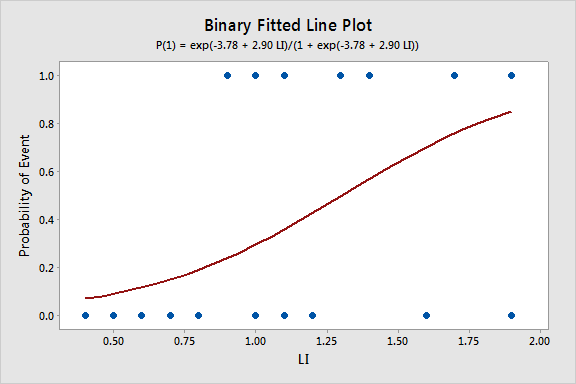
This plot shows a typical logistic regression curve. The outcome is binary (0 or 1), and the model predicts the probability of the event occurring, which follows an S-shaped (sigmoid) curve as the predictor variable (LI) changes.

To solve these issues, we need a function that takes any linear combination of predictors and squashes its output to fit neatly between 0 and 1. This is the core idea behind logistic regression.

The Key Transformation: From Probability to Log-Odds

Logistic regression achieves this "squashing" effect by modeling not the probability directly, but a transformation of the probability. This is done in two steps: first from probability to odds, and then from odds to log-odds (or the logit).

The StatQuest video, "Odds and Log(Odds), Clearly Explained!!!", offers an excellent and intuitive walkthrough of these crucial concepts.

Odds and Log(Odds), Clearly Explained!!!

This video masterfully breaks down the concepts of odds and log-odds, which are the building blocks of logistic regression.

Watch the following segments: The first part clearly distinguishes between probability and odds and shows how they are calculated. The next segment, from log of the odds, explains why taking the logarithm is so useful: it creates a symmetric scale from -∞ to +∞, which is suitable for linear modeling. Finally, the video explicitly connects this to our topic by defining the logit function as the basis for logistic regression.

To summarize the video's key points:

Probability (P): The likelihood of an event, ranging from 0 to 1.
$P (Top Pick)$
Odds: The ratio of the probability of an event happening to the probability of it not happening. Odds range from 0 to +∞.
$Odds = \frac{P ( Top Pick )}{1 - P ( Top Pick )}$
Log-Odds (Logit): The natural logarithm of the odds. This transforms the odds into a scale that ranges from -∞ to +∞, just like the output of a linear regression equation.
$Logit = ln (Odds) = ln (\frac{P ( Top Pick )}{1 - P ( Top Pick )})$

This logit transformation is the "link function" in the Generalized Linear Model (GLM) framework that connects our linear model of predictors to the binomial outcome.

Formulating the Logistic Regression Model

Because the log-odds are on a continuous, unbounded scale, we can now model them with a familiar linear equation:

ln (\frac{P}{1 - P}) = β_{0} + β_{1} X_{1} + β_{2} X_{2} + \dots + β_{k} X_{k}

This is the fundamental equation of a logistic regression model. It states that the log-odds of an event are a linear combination of the predictor variables.

To get back to the probability, $P$ , which is what we actually want to predict, we can rearrange this equation using the inverse of the logit function, which is the sigmoid (or logistic) function:

P = \frac{e ^{β_{0} + β_{1} X_{1} + \dots + β_{k} X_{k}}}{1 + e ^{β_{0} + β_{1} X_{1} + \dots + β_{k} X_{k}}} = \frac{1}{1 + e ^{- (β_{0} + β_{1} X_{1} + \dots + β_{k} X_{k})}}

This equation guarantees that our predicted probability $P$ will always be between 0 and 1. The following diagram illustrates this entire workflow.

This diagram shows the process inside a logistic regression model. The inputs (x), weights (w), and bias (b) are first combined in a linear equation. The result, z, is then passed through a sigmoid function to produce a probability estimate, ŷ, which is then used for classification.

To learn more about the model's structure and the underlying assumptions for its correct formulation, the following resource from Penn State's statistics program is very helpful.

12.1 - Logistic Regression | STAT 462

This text provides a concise mathematical definition of the multiple binary logistic regression model.

Read the initial part of the page, starting from the introduction and continuing down to the formula for the multiple binary logistic regression model. Pay attention to the three different but equivalent ways the model is written: the probability form (with the sigmoid function), the odds form, and the log-odds (logit) form. This reinforces how the different concepts we've discussed fit together mathematically.

A Lingerie Design Example

Let's formulate a model for our specific project. We want to predict the probability that a lingerie piece is a Top_Pick (1 if yes, 0 if no). We believe this depends on three design features:

Lace_Coverage_Pct (a continuous variable from 0 to 100)
Is_Underwired (a binary variable: 1 if yes, 0 if no)
Style_Is_Balconette (a binary variable: 1 if yes, 0 if no)

Our logistic regression model equation would be:

ln (\frac{P ( Top_Pick )}{1 - P ( Top_Pick )}) = β_{0} + β_{1} \cdot Lace_Coverage_Pct + β_{2} \cdot Is_Underwired + β_{3} \cdot Style_Is_Balconette

Here, the $β$ coefficients are estimated from your data using Maximum Likelihood Estimation (MLE), a method you'll be familiar with from your background. The model finds the $β$ values that maximize the likelihood of observing the actual data you have.

Before fitting the model, it's also important to be aware of its assumptions.

Logistic Regression Overview with Example - Statistics By Jim

This article by Jim Frost provides a clear, non-technical list of the main assumptions for logistic regression.

Please read the short section titled Logistic Regression Model Assumptions. The key assumption to note is Linearity in the Logit. This means we assume that for a one-unit change in a predictor, the log-odds of the outcome change by a constant amount, not the probability itself.

Numerical Exercise

Now, let's put this formulation into practice. Suppose you have collected data and used statistical software to fit the model we just defined. The software gives you the following estimated coefficients:

$β_{0}$ (Intercept): -4.0
$β_{1}$ (for Lace_Coverage_Pct): +0.05
$β_{2}$ (for Is_Underwired): +1.5
$β_{3}$ (for Style_Is_Balconette): -0.5

So, your fitted model is:

ln (Odds of Top Pick) = - 4.0 + 0.05 \cdot Lace_Coverage_Pct + 1.5 \cdot Is_Underwired - 0.5 \cdot Style_Is_Balconette

Now, consider a new design you are evaluating:

A non-balconette style (Style_Is_Balconette = 0)
It is underwired (Is_Underwired = 1)
It has 60% lace coverage (Lace_Coverage_Pct = 60)

Your Task:

Calculate the log-odds of this piece being a 'Top Pick' by plugging the values into the equation.
Convert the log-odds into odds. (Hint: Odds = exp(log-odds))
Convert the odds into the final predicted probability. (Hint: Probability = Odds / (1 + Odds))

What is the predicted probability that this new design will be a 'Top Pick'?

Click for a detailed solution.

1. Calculate the Log-Odds:
First, we plug the values for the new design into our fitted model equation:

Log-Odds = - 4.0 + (0.05 \times 60) + (1.5 \times 1) - (0.5 \times 0)

Log-Odds = - 4.0 + 3.0 + 1.5 - 0

Log-Odds = 0.5

2. Convert Log-Odds to Odds:
Next, we exponentiate the log-odds to find the odds:

Odds = e^{0.5} \approx 1.649

This means the odds are about 1.65 to 1 in favor of this piece being a 'Top Pick'.

3. Convert Odds to Probability:
Finally, we convert these odds into a probability:

P (Top Pick) = \frac{Odds}{1 + Odds} = \frac{1.649}{1 + 1.649} = \frac{1.649}{2.649} \approx 0.622

The predicted probability that this new lingerie piece will be a 'Top Pick' is approximately 62.2%.

Conclusion

In this lesson, we transitioned from modeling continuous outcomes with linear regression to modeling binary outcomes with logistic regression. You have learned why OLS is unsuitable for this task and how logistic regression elegantly solves the problem by modeling the log-odds of the outcome.

Key Takeaways:

Logistic regression is used for binary or categorical outcomes, where linear regression fails.
The relationship between predictors and probability is modeled via an S-shaped (sigmoid) curve.
The core of logistic regression is the logit transformation, which converts probability to log-odds: $ln (P / (1 - P))$ .
The logistic regression model assumes a linear relationship between the predictors and the log-odds of the outcome.

We have successfully formulated the model and used it to make a prediction. However, the true power of this technique lies in understanding what the coefficients themselves tell us about the influence of each design feature. In our next lesson, we will focus exclusively on interpreting these coefficients by converting them into odds ratios, a crucial skill for drawing actionable insights from your model.

Recommended resources