QFT in Qiskit: A Small-Qubit Implementation

1. The Anatomy of a QFT Circuit

At its core, the Quantum Fourier Transform is a circuit built from a specific pattern of single- and two-qubit gates. Let's build up the intuition for this pattern, starting from the simplest case.

For a single qubit: The QFT is simply a Hadamard gate. As we've seen before, the H gate transforms the computational basis states $|0⟩$ and $|1⟩$ into the superposition states $|+⟩$ and $|-⟩$, which form the Fourier basis for a 1-qubit system.

For two or more qubits: The circuit becomes more interesting. It involves three main ingredients:

1. Hadamard gates: Applied to each qubit.
2. Controlled Phase Rotation gates: Applied between pairs of qubits.
3. SWAP gates: Applied at the end to correct the qubit ordering.

Let's look at the structure for two qubits.

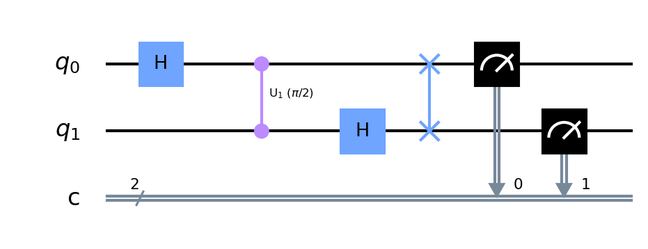
Notice the pattern: a Hadamard is applied to the first qubit, followed by a controlled rotation on the second qubit. Then, a Hadamard is applied to the second qubit. Finally, the qubits are swapped. This pattern generalizes to any number of qubits.

To understand this general structure, the following video provides a clear, step-by-step construction.

As the video explains, the circuit for an n-qubit QFT on qubits $q_0,q_1,\dots ,q_{n-1}$ follows this recipe:

1. Apply a Hadamard gate to $q_0$. Then, for each subsequent qubit $q_j$, apply a controlled-rotation from $q_j$ to $q_0$ with an angle of $\pi /2^j$.
2. Apply a Hadamard gate to $q_1$. Then, for each subsequent qubit $q_j$, apply a controlled-rotation from $q_j$ to $q_1$ with an angle of $\pi /2^{(j-1)}$.
3. Continue this pattern down to the last qubit, which only gets a Hadamard gate.
4. Reverse the order of the qubits using SWAP gates. For example, in a 3-qubit circuit, you would swap $q_0$ and $q_2$.

2. Implementing the QFT in Qiskit

While it's possible to code this entire sequence of gates manually, Qiskit provides a much more convenient way to work with the QFT through its circuit library. This is great for practical use, but we can also use it to verify the structure we just learned.

The QFTGate object in qiskit.circuit.library creates the entire QFT circuit for a specified number of qubits. We can then use the .decompose() method to "look inside" and see the elementary gates it's made of.

Let's explore this in the IBM Quantum Learning resource.

As you'll see in the resource, Qiskit's implementation follows the same logic of Hadamards and controlled-phase rotations. It might look slightly different because Qiskit performs some optimizations to use fewer gates, but the underlying principle is identical. You'll see H gates, CP (Controlled-Phase) gates with decreasing angles, and SWAP gates at the end.

3. A Practical Example: QFT and its Inverse

Now let's use the QFTGate to build and run a circuit. A fundamental property of any unitary transformation, including the QFT, is that it is reversible. If we apply the QFT and then immediately apply its inverse (also known as the adjoint or dagger, QFT${}^{†}$), we should get our original state back. This is a great way to verify our implementation.

Let's test this with a 3-qubit circuit. We'll prepare an arbitrary initial state, say $|101⟩$, apply the QFT, then apply the inverse QFT, and measure the result. We expect to measure $|101⟩$ with 100% probability (ignoring simulator noise).

Here is the Qiskit code to perform this experiment:

from qiskit import QuantumCircuit, transpile
from qiskit_aer import AerSimulator
from qiskit.circuit.library import QFT
from qiskit.visualization import plot_histogram




# --- Setup ---
# We will use a 3-qubit circuit
NUM_QUBITS = 3



# The state we want to prepare is |101>
# Note: Qiskit's bit ordering is q2, q1, q0. So |101> means q2=1, q1=0, q0=1
INITIAL_STATE = '101'




# --- Circuit Construction ---
# Create a quantum circuit with 3 qubits and 3 classical bits
qc = QuantumCircuit(NUM_QUBITS, NUM_QUBITS)




# 1. Prepare the initial state |101>
# Apply an X gate to q0 and q2
qc.x(0)
qc.x(2)
qc.barrier() # Just for visualization




# 2. Apply the Quantum Fourier Transform
# We can get the QFT for 3 qubits from the circuit library
qft_gate = QFT(num_qubits=NUM_QUBITS, name='QFT')
qc.append(qft_gate, range(NUM_QUBITS))
qc.barrier()




# 3. Apply the Inverse Quantum Fourier Transform
# We can get the inverse by calling the .inverse() method
iqft_gate = qft_gate.inverse()
qc.append(iqft_gate, range(NUM_QUBITS))
qc.barrier()




# 4. Measure the qubits
qc.measure(range(NUM_QUBITS), range(NUM_QUBITS))




# Display the circuit
print("Quantum Circuit:")
display(qc.draw("mpl"))




# --- Simulation ---
# Run the circuit on a simulator
simulator = AerSimulator()
transpiled_circuit = transpile(qc, simulator)
result = simulator.run(transpiled_circuit, shots=1024).result()
counts = result.get_counts()




# Display the results
print("\nSimulation Results:")
plot_histogram(counts)

Running the Code:

1. Preparation: We start by applying X gates to qubits 0 and 2 to create the state $|101⟩$.
2. QFT: We create a QFT gate for 3 qubits and append it to our circuit.
3. Inverse QFT: We call .inverse() on our QFT gate to get the inverse transform and append that.
4. Measurement & Results: When you run this code, the histogram of the measurement results should show a single bar at 101, confirming that the QFT followed by its inverse successfully returned the circuit to its initial state.

This simple test gives you a practical feel for how to instantiate, apply, and reverse the QFT in a real Qiskit program.

Conclusion

In this lesson, we bridged the gap between the concept and the practice of the Quantum Fourier Transform. You've seen that this powerful tool is not an indivisible "black box" but is constructed from a clear, repeating pattern of fundamental quantum gates.

Key Takeaways:

• The n-qubit QFT circuit is built from Hadamard gates, a series of controlled-phase rotations with systematically decreasing angles, and SWAP gates at the end to correct qubit ordering.
• In Qiskit, you can inspect this structure by creating a QFTGate from the circuit.library and using the .decompose() method.
• For practical purposes, you can directly append the QFTGate to your circuit.
• The inverse QFT can be obtained using the .inverse() method, which is crucial for algorithms like phase estimation and for verifying your circuits.

Preview of the Next Lesson:

We have now examined all the key components of Shor's algorithm: the classical reduction to period-finding, the creation of a periodic quantum state, and the QFT circuit used to extract that period. In the final lesson of this module, we will put all these pieces together to explain conceptually how Shor's algorithm achieves its famous exponential speedup over classical computers.