Tensor Products for Multi-Qubit States

1. Combining Systems: Beyond Stacking Vectors

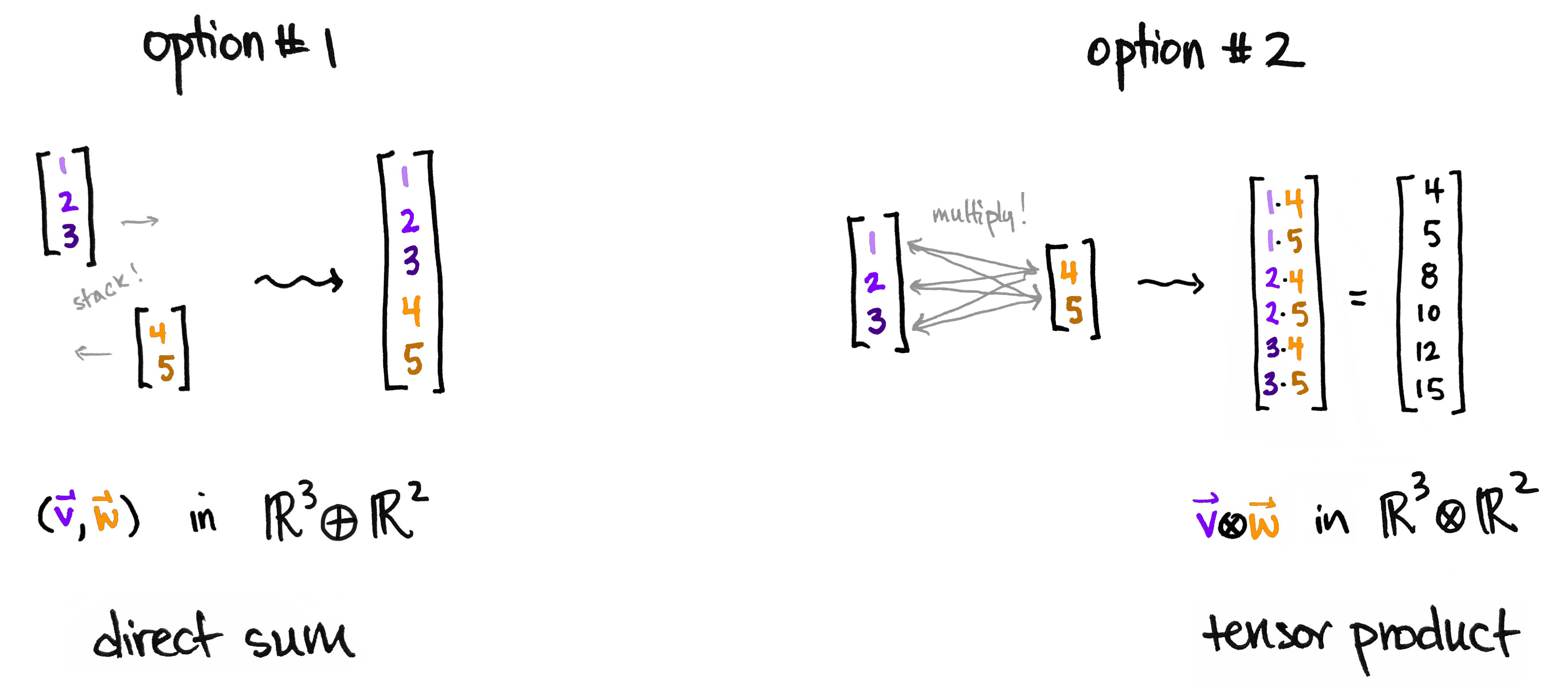
When we combine two quantum systems, we need to create a new state space that accounts for all possible combinations of the original states. A common first guess might be to just stack the state vectors on top of each other (an operation called a direct sum). However, a two-qubit system has four distinct classical states ($|00⟩,|01⟩,|10⟩,|11⟩$), so we need a 4-dimensional vector to represent a superposition of them all.

The correct operation for this is the tensor product, denoted by the symbol $\otimes$. The tensor product creates a new, larger vector space whose dimensions are the product of the original spaces' dimensions (e.g., a 2D space $\otimes$ a 2D space = a 4D space).

The following video provides an excellent conceptual introduction to combining systems, starting with familiar classical ideas before moving to the quantum case.

2. The Mechanics of the Tensor Product

Now, let's look at how the tensor product is calculated. The rule is straightforward: you multiply each element of the first vector by the entire second vector.

This next video offers a very clear, step-by-step demonstration of this calculation for two general single-qubit vectors.

Let's formalize this. Given two single-qubit states:
$|\psi ⟩=\left(\begin{array}{c}{\alpha }_0\\ {\alpha }_1\end{array}\right)\text{and}|\varphi ⟩=\left(\begin{array}{c}{\beta }_0\\ {\beta }_1\end{array}\right)$

Their tensor product $|\psi ⟩\otimes |\varphi ⟩$ is calculated as:
$|\psi ⟩\otimes |\varphi ⟩=\left(\begin{array}{c}{\alpha }_0\\ {\alpha }_1\end{array}\right)\otimes \left(\begin{array}{c}{\beta }_0\\ {\beta }_1\end{array}\right)=\left(\begin{array}{c}{\alpha }_0\left(\begin{array}{c}{\beta }_0\\ {\beta }_1\end{array}\right)\\ {\alpha }_1\left(\begin{array}{c}{\beta }_0\\ {\beta }_1\end{array}\right)\end{array}\right)=\left(\begin{array}{c}{\alpha }_0{\beta }_0\\ {\alpha }_0{\beta }_1\\ {\alpha }_1{\beta }_0\\ {\alpha }_1{\beta }_1\end{array}\right)$

The resulting 4-element vector lives in the two-qubit state space. The entries correspond to the amplitudes of the basis states $|00⟩,|01⟩,|10⟩$, and $|11⟩$, respectively. This is known as lexicographical, or dictionary, ordering.

3. Constructing the Two-Qubit Basis

With the calculation rule in hand, we can now construct the column vectors for the four computational basis states of a two-qubit system. These form the fundamental building blocks for all two-qubit states.

The following video walks through creating each of these four basis vectors.

Here is a summary of the results from the video. Notice how each vector has a '1' in a unique position, confirming they are orthogonal basis vectors for the 4D space.

• State $|00⟩$: This is $|0⟩\otimes |0⟩$.
  $|0⟩\otimes |0⟩=\left(\begin{array}{c}1\\ 0\end{array}\right)\otimes \left(\begin{array}{c}1\\ 0\end{array}\right)=\left(\begin{array}{c}1\cdot 1\\ 1\cdot 0\\ 0\cdot 1\\ 0\cdot 0\end{array}\right)=\left(\begin{array}{c}1\\ 0\\ 0\\ 0\end{array}\right)$

• State $|01⟩$: This is $|0⟩\otimes |1⟩$.
  $|0⟩\otimes |1⟩=\left(\begin{array}{c}1\\ 0\end{array}\right)\otimes \left(\begin{array}{c}0\\ 1\end{array}\right)=\left(\begin{array}{c}1\cdot 0\\ 1\cdot 1\\ 0\cdot 0\\ 0\cdot 1\end{array}\right)=\left(\begin{array}{c}0\\ 1\\ 0\\ 0\end{array}\right)$

• State $|10⟩$: This is $|1⟩\otimes |0⟩$.
  $|1⟩\otimes |0⟩=\left(\begin{array}{c}0\\ 1\end{array}\right)\otimes \left(\begin{array}{c}1\\ 0\end{array}\right)=\left(\begin{array}{c}0\cdot 1\\ 0\cdot 0\\ 1\cdot 1\\ 1\cdot 0\end{array}\right)=\left(\begin{array}{c}0\\ 0\\ 1\\ 0\end{array}\right)$

• State $|11⟩$: This is $|1⟩\otimes |1⟩$.
  $|1⟩\otimes |1⟩=\left(\begin{array}{c}0\\ 1\end{array}\right)\otimes \left(\begin{array}{c}0\\ 1\end{array}\right)=\left(\begin{array}{c}0\cdot 0\\ 0\cdot 1\\ 1\cdot 0\\ 1\cdot 1\end{array}\right)=\left(\begin{array}{c}0\\ 0\\ 0\\ 1\end{array}\right)$

Any two-qubit state can be written as a linear combination (a superposition) of these four basis vectors.

4. Product States vs. Entangled States

A crucial concept that arises from the tensor product is the distinction between product states and entangled states.

• A product state is any multi-qubit state that can be written as the tensor product of individual, single-qubit states. These systems are independent.
• An entangled state is a multi-qubit state that cannot be factored into a tensor product of individual qubit states. The qubits in an entangled state are correlated in a way that has no classical equivalent.

The most famous entangled state is the Bell state, $|{\Phi }^{+}⟩=\frac{1}{\sqrt{2}}(|00⟩+|11⟩)$. Its state vector is:
$|{\Phi }^{+}⟩=\frac{1}{\sqrt{2}}\left(\begin{array}{c}1\\ 0\\ 0\\ 1\end{array}\right)$
It is impossible to find two single-qubit states $|\psi ⟩$ and $|\varphi ⟩$ such that $|\psi ⟩\otimes |\varphi ⟩=|{\Phi }^{+}⟩$. The following video explains why.

5. Tensor Products in Qiskit

As you're keen on practical implementation, let's see how to do this in Qiskit. Qiskit's Statevector class makes this very easy.

Here's a quick example based on the reading. To create the $|01⟩$ state vector:

from qiskit.quantum_info import Statevector




# Create state vectors for |0> and |1>
zero = Statevector.from_label("0")
one = Statevector.from_label("1")




# Compute the tensor product |0> ⊗ |1> using the ^ operator
psi = zero ^ one




# Display the resulting state vector
print("State |01>:")
display(psi.draw("latex"))
print(psi.data)

Running this code would show you the state $|01⟩$ and its underlying array [0.+0.j, 1.+0.j, 0.+0.j, 0.+0.j], which matches the vector $(0,1,0,0)$ we derived manually.

Conclusion

Today, we've made a significant leap from describing single qubits to describing multi-qubit systems. The tensor product is the fundamental tool that allows us to build these larger, more complex state spaces.

Key Takeaways:

• To represent a multi-qubit system, we use the tensor product ($\otimes$) to combine the state vectors of individual qubits.
• The dimension of the combined state space is the product of the individual dimensions. For $n$ qubits, the state vector has $2^n$ elements.
• The calculation follows a clear rule: multiply each element of the first vector by the entire second vector to form the new, larger vector.
• A multi-qubit state that can be factored into a tensor product of single-qubit states is a product state. If it cannot be factored, it is an entangled state.

Preview of the Next Lesson:
Now that we understand qubit states (single and multi-qubit) and the matrix operations that act on them, we'll turn our attention to a crucial property of those matrices. In the next lesson, we will explore what it means for a matrix to be unitary and why this property guarantees that quantum evolution is reversible—a key feature that distinguishes quantum gates from many classical logic gates.