Grover's Algorithm: Oracle and Diffusion Operator

1. The Oracle: Marking the Target

The first step in Grover's algorithm isn't to find the answer, but simply to "mark" it. This is the job of the oracle. The oracle is a quantum black box that knows which item is the "winner" but doesn't reveal it directly. Instead, it applies a unique signature to the winning state: it flips its phase.

Recall that a quantum state is a superposition of basis states, each with a complex amplitude. For an $n$-qubit system, an arbitrary state can be written as:

The oracle, $U_w$, is an operator that acts on this state. If $|w⟩$ is the winning state we're searching for, the oracle flips its amplitude's sign:

Initially, the algorithm starts in a uniform superposition $|s⟩$, where all amplitudes are equal, ${\alpha }_x=1/\sqrt{N}$. After applying the oracle, the amplitude of the winning state becomes $-1/\sqrt{N}$, while all others remain unchanged.

To see how this works, let's watch a short clip that demonstrates the oracle's function.

How is an Oracle Built?

You might wonder how we can build an oracle that "knows" the answer without us knowing it first. This is a crucial point. Grover's algorithm is useful for problems where verifying a solution is easy, even if finding it is hard.

The oracle is the quantum implementation of a classical verification function, $f(x)$, where $f(x)=1$ if $x$ is the solution and $f(x)=0$ otherwise. Using a technique called phase kickback (which you've seen in the Bernstein-Vazirani algorithm), we can translate this classical function into a quantum operator that applies a phase of $(-1{)}^{f(x)}$ to the state $|x⟩$.

For a deeper dive into this concept, let's turn to a more detailed explanation.

At this point, the probability of measuring the winning state is unchanged, since $|-1/\sqrt{N}{|}^2=|1/\sqrt{N}{|}^2$. The phase flip is invisible to a direct measurement. Its power lies in how it sets up the next step: amplification.

2. The Diffusion Operator: Amplifying the Marked State

After the oracle marks the target state with a negative phase, the diffusion operator, $U_s$, performs its magic. Its job is to amplify the amplitude of the marked state while shrinking all others. It achieves this through a clever operation often described as "inversion about the mean."

Let's break this down:

1. After the oracle, the average amplitude of all states has been slightly lowered because of the one negative amplitude.
2. The amplitudes of the "loser" states are all slightly above this new average.
3. The amplitude of the "winner" state is far below the average.
4. The diffusion operator reflects every amplitude across the average. The loser states, being just above the average, are reflected to be just below it (their amplitudes decrease). The winner state, being far below the average, is reflected to be far above it (its amplitude increases significantly).

This process is best understood geometrically. In the last lesson, we saw a preview of this. Let's re-watch that segment with our new knowledge of the oracle.

How is the Diffusion Operator Built?

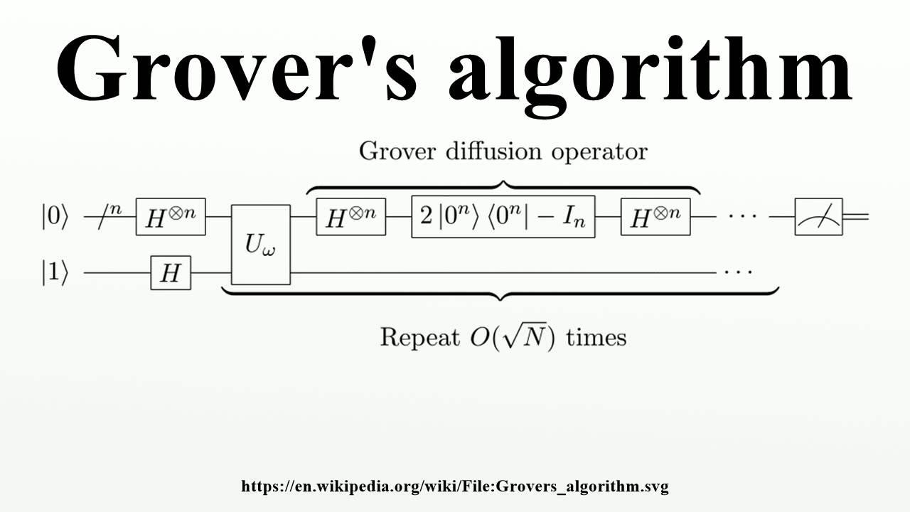
The diffusion operator, $U_s$, is a reflection about the initial uniform superposition state $|s⟩$. Its mathematical form is $U_s=2|s⟩⟨s|-I$. While this looks abstract, its circuit implementation is surprisingly elegant and relies on the Hadamard gate.

The operator is constructed as follows:

1. Apply Hadamard gates to all qubits. This transforms the state from the superposition basis back to the computational basis, specifically mapping $|s⟩$ to $|0...0⟩$.
2. Apply an operation that flips the phase of the $|0...0⟩$ state but leaves all other states unchanged.
3. Apply Hadamard gates again to transform back to the superposition basis.

This sequence effectively performs the "inversion about the mean" operation.

The following diagram shows a complete Grover iteration, which consists of one application of the oracle followed by one application of the diffusion operator.

3. A Concrete Example: 2-Qubit Search

Let's walk through the state evolution for a simple 2-qubit search where $N=4$ and the winning state is $|01⟩$. This will solidify how the oracle and diffuser work together. The following steps are based on the excellent example in the IBM Quantum Learning resource.

1. Initialization:
We start in the uniform superposition state $|s⟩$, created by applying Hadamard gates to $|00⟩$.

All states have an amplitude of $1/2$ and a measurement probability of $1/4$.

2. Apply Oracle $U_w$:
The oracle for the winning state $|01⟩$ flips its phase.

The phase of $|01⟩$ is now negative. Measurement probability is still uniform.

3. Apply Diffusion Operator $U_s$:
The diffusion operator now performs inversion about the mean. The average amplitude is $\frac{1}{2}(1/2-1/2+1/2+1/2)=1/4$.

• The "loser" states ($|00⟩,|10⟩,|11⟩$) have an amplitude of $1/2$. Reflecting this about the mean $1/4$ gives an amplitude of $0$.
• The "winner" state ($|01⟩$) has an amplitude of $-1/2$. Reflecting this about the mean $1/4$ gives an amplitude of $1$.

The final state after one full Grover iteration is:

In this specific case of $N=4$, a single iteration is enough to rotate the state vector perfectly to the solution. A measurement will now yield $|01⟩$ with 100% probability. For larger $N$, the rotation per step is much smaller, and multiple iterations are needed.

Conclusion

In this lesson, we dissected the two fundamental components that power Grover's algorithm. We saw that the process is a well-defined, two-step dance of marking and amplifying.

Key Takeaways:

• The Oracle ($U_w$): This operator "marks" the winning state(s) by applying a phase flip (multiplying the amplitude by -1). It's the quantum embodiment of a classical verification function.
• The Diffusion Operator ($U_s$): This operator performs an "inversion about the mean," which amplifies the amplitude of the marked state and suppresses the others.
• Geometric Interpretation: Together, the oracle (a reflection) and the diffusion operator (a second reflection) combine to perform a rotation, systematically moving the quantum state closer to the solution with each iteration.

Preview of the Next Lesson:
For a search space of size $N=4$, we saw that one iteration was perfect. But what about for $N=1,000,000$? Is one iteration enough? And what happens if we do too many? In our next lesson, we will answer this by learning how to determine the optimal number of iterations for a Grover search. We will then be ready to construct and simulate the complete algorithm in Qiskit.