Utility Maximization with Budget Constraints

1. The Budget Constraint: The Realm of the Possible

A consumer's choices are limited by two main factors: their income and the prices of goods. The budget constraint is the mathematical representation of this limitation. It defines the set of all consumption bundles a consumer can afford.

To understand how to build and interpret this constraint, please watch the following segments from a lecture by Professor Jonathan Gruber. He will introduce the concept, write out the equation, and explain its graphical representation.

As you saw in the video, for a simple world with two goods, say good $x_1$ and good $x_2$, with prices $p_1$ and $p_2$ respectively, and a given income $I$, the budget constraint is formally written as:

$p_1{x}_1+p_2{x}_2\le I$

This inequality states that total expenditure cannot exceed income. Economists often make a simplifying assumption called non-satiation, which means "more is always better." Under this assumption, a rational consumer will always spend their entire income to maximize their satisfaction. The budget constraint thus becomes an equality:

$p_1{x}_1+p_2{x}_2=I$

This equation defines the budget line.

The key features of the budget line are its intercepts and its slope:

• Intercepts: The points where the line hits the axes. The vertical intercept is $I/p_2$ and the horizontal intercept is $I/p_1$. Each represents the maximum amount of one good you could buy if you spent your entire income on it.
• Slope: If we rearrange the budget line equation to solve for $x_2$, we get: $x_2=\frac{I}{p_2}-\frac{p_1}{p_2}{x}_1$. The slope is $-\frac{p_1}{p_2}$.

The slope represents the opportunity cost of consuming one good in terms of the other. It's the rate at which the market allows you to trade good 2 for good 1. This is also called the Marginal Rate of Transformation (MRT).

2. The Objective: Utility Maximization

Now that we've defined the consumer's constraints, let's turn to their objective. In economics, we assume consumers aim to maximize their utility, which is a measure of satisfaction or happiness derived from consumption. We represent this with a utility function, $U(x_1,x_2)$.

The utility function is visualized using indifference curves—curves along which every point (a consumption bundle) provides the same level of utility. The consumer's goal is to reach the highest possible indifference curve, given their budget constraint.

This leads to the core of the consumer's problem: finding the point on the budget line that lies on the highest attainable indifference curve. This occurs at a point of tangency.

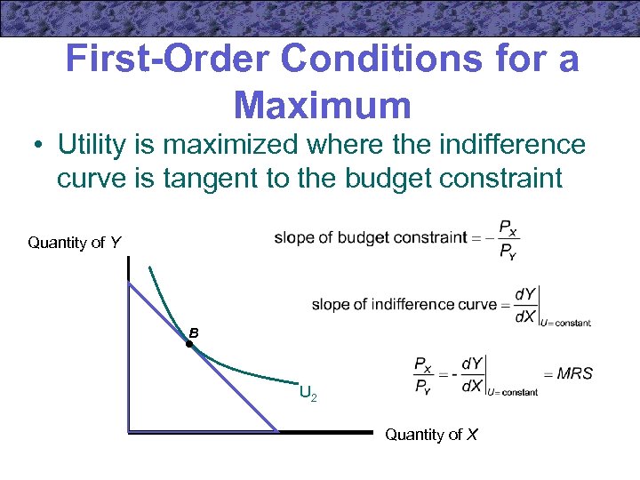
At the point of tangency, the slope of the indifference curve is equal to the slope of the budget line.

• The slope of the indifference curve is the Marginal Rate of Substitution (MRS). It represents the rate at which the consumer is willing to trade one good for the other while maintaining the same level of utility. Mathematically, $MRS=-\frac{\partial U/\partial x_1}{\partial U/\partial x_2}=-\frac{M{U}_1}{M{U}_2}$.
• The slope of the budget line is the price ratio, $-\frac{p_1}{p_2}$.

Therefore, the condition for utility maximization is:
$\text{MRS}=\frac{p_1}{p_2}⟹\frac{M{U}_1}{M{U}_2}=\frac{p_1}{p_2}$
This can be rearranged into the "bang for the buck" equation you heard in the first video: $\frac{M{U}_1}{p_1}=\frac{M{U}_2}{p_2}$. The marginal utility per dollar spent should be equal across all goods.

3. Formalizing the Problem: Constrained Optimization

We can now state the consumer's utility maximization problem in a formal, mathematical way. This structure is analogous to many problems in physics where you seek to optimize a quantity (like energy or action) subject to a set of constraints.

The problem is:
Maximize $U(x_1,x_2)$
Subject to $p_1{x}_1+p_2{x}_2=I$

This is a classic constrained optimization problem. As you've likely encountered in your physics studies (for example, in classical mechanics), the standard tool for solving such problems is the Lagrangian method.

For a deeper dive into the mathematical setup, please read the following section from a set of lecture notes. It formalizes the problem and introduces the Lagrangian.

As the notes detail, we construct the Lagrangian function, $\mathcal{L}$, by combining the objective function and the constraint:

$\mathcal{L}(x_1,x_2,\lambda )=U(x_1,x_2)+\lambda (I-p_1{x}_1-p_2{x}_2)$

Here, $\lambda$ (lambda) is the Lagrange multiplier. To find the optimal consumption bundle $(x_1^{\ast },x_2^{\ast })$, we would take the partial derivatives of $\mathcal{L}$ with respect to $x_1$, $x_2$, and $\lambda$, and set them equal to zero. These are the first-order conditions:

1. $\frac{\partial \mathcal{L}}{\partial x_1}=\frac{\partial U}{\partial x_1}-\lambda p_1=0⟹M{U}_1=\lambda p_1$
2. $\frac{\partial \mathcal{L}}{\partial x_2}=\frac{\partial U}{\partial x_2}-\lambda p_2=0⟹M{U}_2=\lambda p_2$
3. $\frac{\partial \mathcal{L}}{\partial \lambda }=I-p_1{x}_1-p_2{x}_2=0$

Notice that combining the first two conditions by dividing them gives us back our familiar tangency condition: $\frac{M{U}_1}{M{U}_2}=\frac{p_1}{p_2}$. The third condition simply ensures that the solution lies on the budget line.

The Lagrange multiplier, $\lambda$, has a very important economic interpretation: it represents the marginal utility of income—the additional utility gained from one extra dollar of income.

Conclusion

In this lesson, we have laid the complete groundwork for analyzing consumer choice. We have formally defined the consumer's utility maximization problem.

Key Takeaways:

• A consumer's decision is a constrained optimization problem.
• The constraint is the budget line ($p_1{x}_1+p_2{x}_2=I$), which describes the feasible consumption bundles. Its slope, $-p_1/p_2$, represents the market trade-off or opportunity cost.
• The objective is to maximize a utility function $U(x_1,x_2)$, which represents the consumer's preferences.
• The problem is formally stated as maximizing $U(x_1,x_2)$ subject to the budget constraint.
• The Lagrangian is the mathematical tool used to set up and solve this problem: $\mathcal{L}=U(x_1,x_2)+\lambda (I-p_1{x}_1-p_2{x}_2)$.

You are now able to formulate the problem. In our next lesson, we will take the next logical step: we will use the Lagrangian method to solve this problem for specific utility functions and derive the consumer's optimal consumption bundle.