The Kinked Demand Curve Model

The Central Puzzle: Price Rigidity

A defining characteristic of many oligopolistic markets is price stability. While costs of labor or raw materials may fluctuate, firms are often reluctant to alter their prices. Why would a profit-maximizing firm not adjust its price when its costs change? The kinked demand curve model, developed by economist Paul Sweezy, offers one explanation rooted in the strategic interdependence we studied previously.

The model rests on a crucial set of assumptions about how a firm expects its competitors to react to its pricing decisions. This is often termed behavioral asymmetry.

As the reading explains, the model's core logic hinges on two pessimistic assumptions a firm makes about its rivals:

1. If a firm increases its price: It assumes its rivals will not follow suit. They will keep their prices lower to attract the firm's customers.
2. If a firm decreases its price: It assumes its rivals will follow, cutting their own prices to prevent losing market share.

These assumptions are not about collusion but about non-cooperative, self-interested reactions in a market with high interdependence.

Constructing the Kinked Demand Curve

These two assumptions mean the firm perceives its demand curve differently depending on whether it raises or lowers its price from the current prevailing price, let's call it $P^{\ast }$.

To visualize this, let's watch a segment that explains how these rival reactions create different elasticities of demand.

Let's break down the logic from the video:

• Above the current price $P^{\ast }$: If the firm raises its price, rivals do not follow. Customers have many lower-priced alternatives, so they will switch away in large numbers. A small price increase leads to a large drop in quantity demanded. Therefore, the demand curve is relatively elastic above $P^{\ast }$.
• Below the current price $P^{\ast }$: If the firm lowers its price, rivals match the cut. The firm does not gain significant market share from its competitors. It only gains a small increase in sales from the overall market expansion due to the lower price. Therefore, the demand curve is relatively inelastic below $P^{\ast }$.

The firm's perceived demand curve is a composite of these two scenarios. It is the elastic curve for prices above $P^{\ast }$ and the inelastic curve for prices below $P^{\ast }$. The junction of these two segments at the prevailing price $P^{\ast }$ creates the characteristic "kink."

The following diagram, often called the Sweezy demand curve, illustrates this concept perfectly. It shows two underlying demand curves: $D_1$, which applies when rivals hold their price constant (the elastic segment), and $D_2$, which applies when rivals match price changes (the inelastic segment). The firm's actual perceived demand curve, $D_S$, is the combination of the relevant portions of each.

The Discontinuous Marginal Revenue Curve and Its Implication

The kink in the demand curve has a critical consequence for the firm's marginal revenue (MR) curve. As you know, the MR curve's position depends on the demand curve. Since the demand curve is piecewise (composed of two different linear segments), the MR curve will also be piecewise.

Specifically, at the quantity corresponding to the kink ($Q_0$ in the diagram above), the marginal revenue curve will have a vertical discontinuity, or a gap.

• The upper portion of the MR curve corresponds to the more elastic segment of the demand curve.
• The lower portion of the MR curve corresponds to the more inelastic segment of the demand curve.

This discontinuous MR curve is the key to explaining price rigidity.

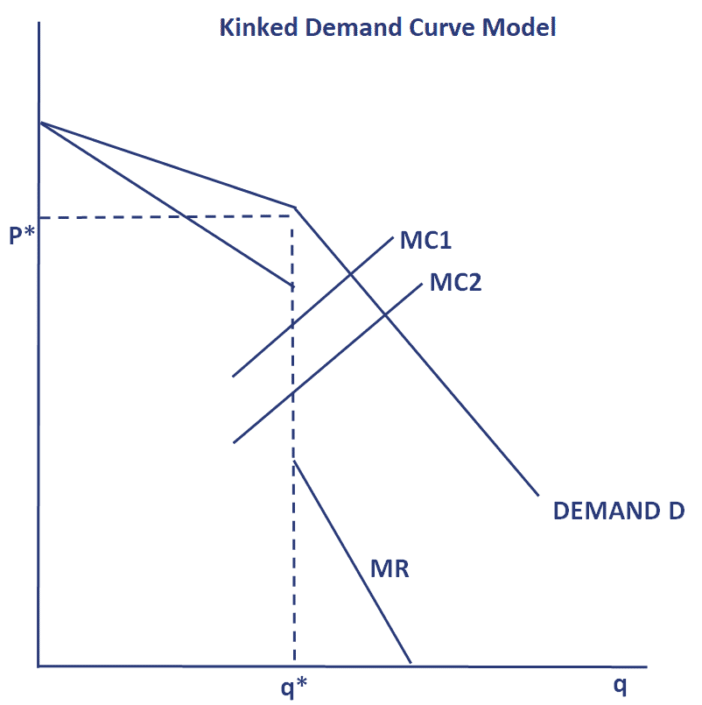
Recall the profit-maximization rule: a firm produces at the quantity where marginal cost (MC) equals marginal revenue (MR).

As the "Kinked Demand Curve Model" graph shows, the firm's MC curve can shift up or down within the vertical gap of the MR curve (e.g., from MC1 to MC2). Because the intersection point of MC and MR is still within this vertical range, the profit-maximizing output level remains unchanged at $q^{\ast }$. The firm continues to charge the price $P^{\ast }$ that corresponds to this quantity on the demand curve.

Let's watch a short video segment that summarizes this final piece of the model.

This is the central prediction of the model: for an oligopolistic firm facing a kinked demand curve, small-to-moderate changes in marginal costs will not trigger a change in price. This provides a theoretical justification for the observed "sticky prices" in these markets.

It is worth noting one critique of this model: it explains why an existing price might be stable, but it does not explain how that price was established in the first place. Nonetheless, it remains a powerful illustration of how strategic assumptions about rival behavior can shape market outcomes.

Conclusion

In this lesson, we have dissected the kinked demand curve model to understand its explanation for price rigidity in oligopolies. We moved from the core behavioral assumptions to the construction of the kinked demand curve and, finally, to its key implication for the marginal revenue curve.

Key Takeaways:

• The kinked demand curve model assumes firms expect an asymmetric response from rivals: rivals will match price cuts but will not match price increases.
• This asymmetry creates a kink in the firm's perceived demand curve at the prevailing price. Demand is relatively elastic above the kink and relatively inelastic below it.
• The kink in the demand curve causes a vertical discontinuity or gap in the marginal revenue curve.
• This MR gap explains price rigidity, as shifts in the marginal cost curve within this gap do not alter the profit-maximizing price and quantity.

In our next lesson, we will build directly on this foundation. Having understood why the marginal revenue curve is segmented, we will proceed to calculate the segmented marginal revenue curve given a specific kinked demand function. This will allow us to apply your quantitative skills to determine the precise range over which marginal costs can fluctuate without affecting the market price.