Marshall-Lerner Condition and the J-Curve Effect

The Ambiguous Effect of a Currency Depreciation

At first glance, the effect of a currency depreciation seems straightforward. If the pound depreciates, UK exports become cheaper for foreigners, and foreign imports become more expensive for UK residents. This should lead to a rise in the quantity of exports sold and a fall in the quantity of imports bought, presumably improving the current account balance (the value of exports minus the value of imports).

However, this is not the full story. The trade balance is measured in value, not just quantity. A depreciation means that while the UK sells more exports, it receives less foreign currency for each unit sold. Similarly, while it buys fewer imports, it pays more in domestic currency for each unit it still imports. There are two competing effects:

1. The Quantity Effect: The change in the volume of exports and imports.
2. The Price (or Valuation) Effect: The change in the value of each unit traded.

The Marshall-Lerner condition is the rule that tells us which effect will dominate.

To start, let's get a clear definition of the condition and a recap of its context.

As the video states, for a depreciation to improve the current account, the demand for exports and imports must be sufficiently responsive to the price change. Formally, the Marshall-Lerner condition states that, starting from a position of balanced trade, a currency depreciation will improve the trade balance if the sum of the absolute values of the price elasticities of demand for exports ($|{ϵ}_X|$) and imports ($|{ϵ}_M|$) is greater than one.

Let's now derive this condition formally. Your background in statistics and preference for mathematical rigor will be very useful here.

Mathematical Derivation of the Condition

To prove why this condition holds, we can model the trade balance and use calculus to see how it changes with the exchange rate. We'll use the Wikipedia article on the topic, which provides a clear and direct derivation.

Let's recap the core of that derivation. The trade surplus ($TB$), measured in domestic currency, is the value of exports ($X$) minus the value of imports ($eM$), where $e$ is the exchange rate (domestic currency per unit of foreign currency) and $M$ is the quantity of imports.

Taking the derivative with respect to $e$ tells us how the trade balance changes as the currency depreciates (as $e$ rises). After several algebraic steps shown in the reading, we arrive at:

(Note: Wikipedia's derivation defines ${ϵ}_x$ as the elasticity of exports w.r.t the exchange rate, which is positive, and ${ϵ}_m$ as the elasticity of imports w.r.t the exchange rate, which is negative. To express this using the standard convention of negative price elasticities, we would write $|{ϵ}_x|+|{ϵ}_m|>1$.)

For the trade balance to improve with depreciation, $\frac{dTB}{de}$ must be positive. Starting from balanced trade ($X=eM$), this occurs if and only if the Marshall-Lerner condition is satisfied.

A Numerical Application

Now, let's solidify this with a numerical example. It's often most instructive to see what happens when a condition is not met. The next video walks through a scenario where elasticities are low, and a depreciation actually worsens the trade balance.

As the video demonstrates, because the sum of the absolute elasticities ($0.7+0.5=1.2$) is greater than 1, the Marshall-Lerner condition is met. However, the video's narrator makes a mistake in his initial setup by stating the average must be greater than one, which is incorrect. The sum must be greater than one. Let's re-examine his numbers correctly.

His calculation shows:

• Initial State: Export Revenue = £100, Import Spend = £100. Trade Balance = £0.
• After 10% Depreciation:
  • Exports: The price falls by 10% (to £0.90). Quantity demanded rises by 7% (from 100 to 107 units). New Export Revenue = 107 * 0.90 = £96.30.
  • Imports: The price rises by 10% (to £1.10). Quantity demanded falls by 5% (from 100 to 95 units). New Import Spend = 95 * 1.10 = £104.50.
• Final State: New Trade Balance = £96.30 - £104.50 = -£8.20.

The trade balance worsened from £0 to a deficit of £8.20. Even though the sum of elasticities was 1.2, the trade balance worsened. Why? This is because the derivation we studied assumed an initial balance of trade. The video's calculation also implicitly starts from a balance, but the result shows a worsening. The nuance here is that the simple condition ${ϵ}_X+{ϵ}_M>1$ applies cleanly when measured in foreign currency or when starting from a perfect balance. When measured in domestic currency with significant trade flows, the valuation effects can be more complex, as shown in the general formula from the Wikipedia derivation. The key takeaway from the video, however, remains valid: when elasticities are low, the negative price effect can easily dominate the positive quantity effect.

Elasticity Dynamics and the J-Curve

So, what determines these elasticities? A key factor is time. In the short run, it's difficult for consumers and firms to change their buying habits. Many import/export deals are governed by long-term contracts. This means demand is relatively inelastic in the short run. Over time, as contracts expire and people find new alternatives, demand becomes more elastic.

This dynamic—where the Marshall-Lerner condition may fail in the short run but hold in the long run—produces a distinctive pattern in the trade balance following a depreciation. This is known as the J-Curve effect.

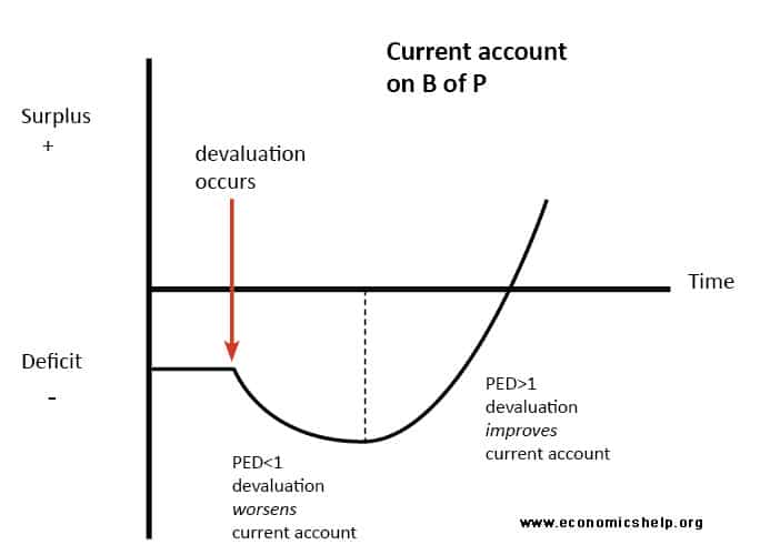
The graph shows that immediately after a currency depreciation:

1. The current account balance worsens. This is the initial part of the "J". Here, prices have changed, but quantities are fixed due to contracts and habit. The negative price/valuation effect dominates. The MLC is not satisfied.
2. Over time, the current account balance improves. This is the upward-sloping part of the "J". Consumers and firms respond to the new prices, increasing export quantities and decreasing import quantities. The positive quantity effect begins to dominate. The MLC becomes satisfied.

Let's watch the final part of the video, which explains and illustrates this J-Curve.

This dynamic is a critical piece of real-world analysis. A government or central bank that engineers a currency devaluation to fix a trade deficit must be patient; things are likely to get worse before they get better.

Conclusion

In this lesson, we have explored the complex relationship between currency values and the trade balance. You've seen that the intuitive idea that "a weaker currency helps the trade balance" is conditional, and you've learned the formal tools to analyze that condition.

Key Takeaways:

• A currency depreciation has two opposing effects on the trade balance: a quantity effect (which is positive) and a price/valuation effect (which is negative).
• The Marshall-Lerner condition ($|{ϵ}_X|+|{ϵ}_M|>1$) states that for a depreciation to improve the trade balance (from an initial balance), the sum of demand elasticities for exports and imports must be greater than one.
• We can formally derive this condition by analyzing the derivative of the trade balance equation with respect to the exchange rate.
• The J-Curve effect describes the dynamic path of the trade balance over time. It initially worsens due to low short-run elasticities (contracts, habits) and then improves as elasticities rise in the long run.

This lesson concludes our module on International Trade and Finance. We've covered how countries benefit from trade, the effects of protectionism, how international transactions are recorded, and how exchange rates are determined and, in turn, affect the economy.

In our next lesson, we will begin a new module, shifting our focus to the domestic Financial System. We'll start by learning how to calculate the price of a bond, a fundamental building block for understanding how interest rates are determined in the wider economy and how monetary policy operates.