In our previous lesson, we mastered the t-test, a powerful tool for comparing the means of continuous variables between one or two groups. This is essential for questions like, "Does this drug lower blood pressure more than a placebo?" But clinical research often involves categorical data. For instance, you might need to determine if there's a relationship between a patient's smoking status (smoker vs. non-smoker) and their treatment outcome (improved vs. not improved). The t-test is not suitable for this kind of data.
This lesson introduces the statistical tool designed for precisely this scenario: the chi-square () test of independence. You will learn how to use this test to determine whether a statistically significant association exists between two categorical variables. We will cover the entire workflow, from formulating hypotheses and visualizing the data to performing the test in R, interpreting the results, and quantifying the strength of any discovered relationship.
1. The Logic: Observed vs. Expected Frequencies
The t-test works by comparing means. The chi-square test works by comparing counts, or frequencies. The core idea is to compare the frequencies we actually observe in our data with the frequencies we would expect to see if there were no relationship between the variables at all.
Imagine you are studying the relationship between a new teaching method (New vs. Standard) and student exam results (Pass vs. Fail). You collect data and put it in a contingency table:
| Method | Pass | Fail | Total |
|---|---|---|---|
| New | 40 | 10 | 50 |
| Standard | 30 | 20 | 50 |
| Total | 70 | 30 | 100 |
These are your observed frequencies.
Now, if there were no relationship between the teaching method and the outcome (this is our null hypothesis), the proportion of students passing and failing would be the same for both methods. Overall, 70% of students passed (70/100) and 30% failed (30/100). So, we would expect:
- New Method Group: 70% of 50 = 35 pass, 30% of 50 = 15 fail.
- Standard Method Group: 70% of 50 = 35 pass, 30% of 50 = 15 fail.
These are your expected frequencies. The chi-square test quantifies the difference between the observed and expected tables. A large difference suggests the variables are not independent, and there might be a real association.
This leads to our hypotheses:
- Null Hypothesis (): There is no association between the two variables (they are independent).
- Alternative Hypothesis (): There is an association between the two variables (they are dependent).
5 Chi-squared Test – Notes on Statistics with R (SwR) - Bookdown
This online book provides a detailed walkthrough of the chi-square test. To solidify the core logic, please read the sections on the underlying concepts.
Start at the section titled Comparing groups and read through the subsections on Observed and Expected values. Then, review the list of assumptions. This will clarify the theoretical foundation before we start coding.
2. Performing the Chi-Square Test in R
Let's put this into practice. We'll use the built-in iris dataset. Since the chi-square test requires categorical variables, we will first create a new categorical variable called size based on the Sepal.Length. This mimics a common real-world analysis task where you might categorize a continuous measurement (like blood pressure) into groups (e.g., 'Normal', 'High').
Step 1: Prepare and Explore the Data
First, ensure you have the necessary packages installed and loaded. We'll continue using rstatix for its tidy workflow, and we'll add janitor for its excellent table-making functions.
# install.packages("tidyverse")
# install.packages("rstatix")
# install.packages("janitor") # For creating nice frequency tables

library(tidyverse)
library(rstatix)
library(janitor)


# Create a categorical variable from a continuous one
iris_cat <- iris %>%
  mutate(size = case_when(
    Sepal.Length < median(Sepal.Length) ~ "small",
    TRUE ~ "big"
  ))
Now, let's create a contingency table to see the observed counts of each Species in each size category. The tabyl() function from janitor is perfect for this.
# Create a contingency table
contingency_table <- iris_cat %>%
  tabyl(Species, size)

contingency_table
This will produce a clean frequency table. Before testing, it's always good practice to visualize the relationship. A stacked bar chart showing proportions is an effective way to do this.
ggplot(iris_cat, aes(x = Species, fill = size)) +
  geom_bar(position = "fill") +
  labs(
    y = "Proportion",
    title = "Proportion of 'big' vs 'small' flowers by Species"
  )
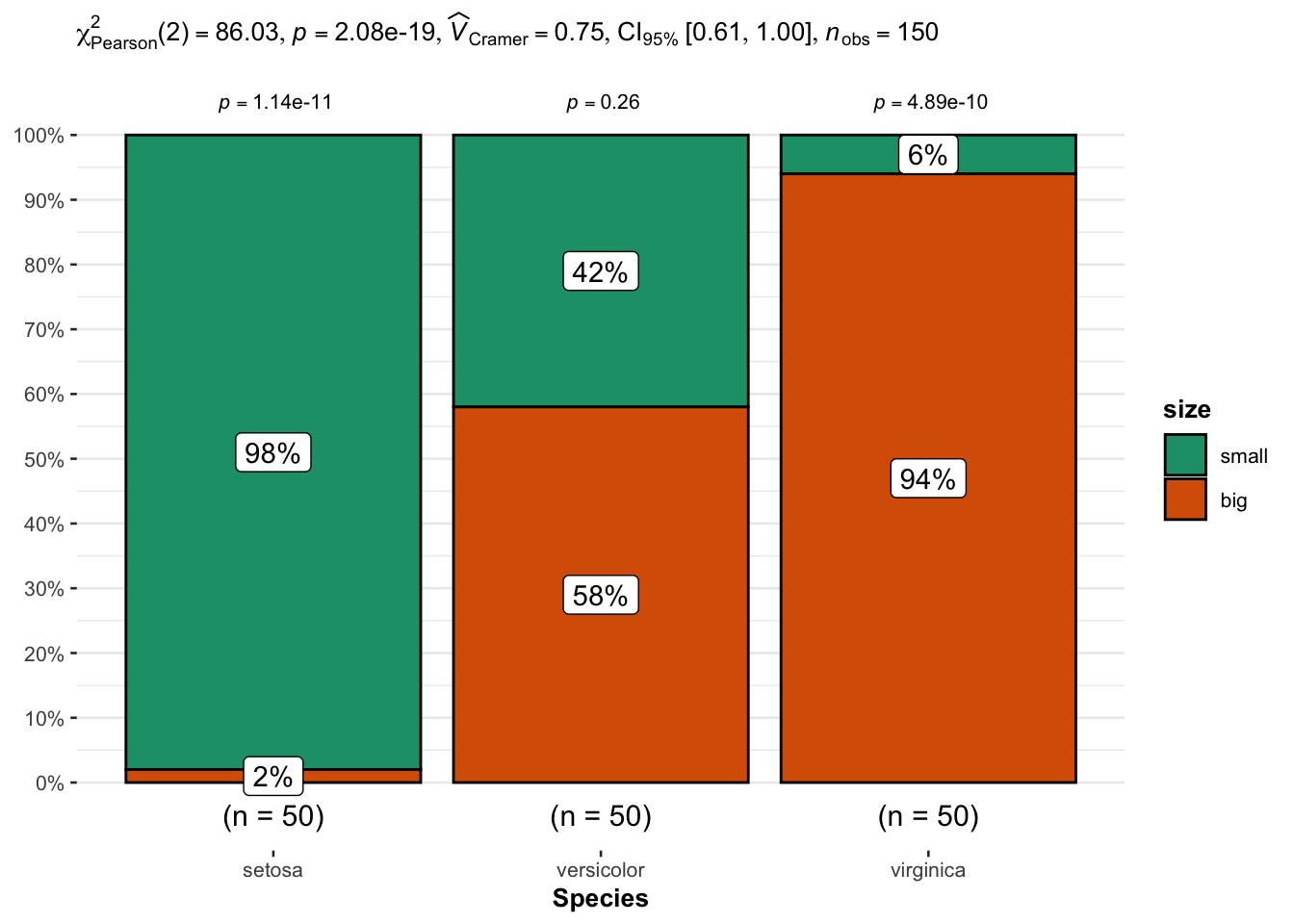
The plot visually suggests that the distribution of 'small' and 'big' flowers is very different across the species. Now, let's formally test if this association is statistically significant.
Step 2: The Test and Interpretation
We will use the chisq_test() function from rstatix, which follows the familiar formula syntax.
# Perform the chi-square test
test_result <- iris_cat %>%
  chisq_test(Species ~ size)


# View the result
test_result
The output will give you three key pieces of information:
statistic: This is the chi-square () value itself. It's a single number that summarizes the total difference between your observed and expected cell counts. The larger the value, the greater the discrepancy.df: The degrees of freedom. For a chi-square test, this is calculated as(number of rows - 1) * (number of columns - 1). It defines the shape of the chi-square distribution used to calculate the p-value.p: The p-value. This is the probability of observing a statistic as large as, or larger than, the one calculated, assuming the null hypothesis (no association) is true.
Our conclusion rests on the p-value. If p is less than our chosen significance level (typically 0.05), we reject the null hypothesis. We conclude that there is a statistically significant association between the two variables. In our iris example, the p-value will be extremely small, confirming our visual impression from the plot.
Step 3: Checking Assumptions
The primary assumption of the chi-square test is that the sample size is large enough. The rule of thumb is: at least 80% of the cells in the expected frequency table must have a count of 5 or more, and no cell should have an expected count less than 1.
The rstatix package makes this easy. The test object we created, test_result, already contains the expected counts. You can access them directly:
test_result$expected
If the assumption is violated (which might happen with small sample sizes or many categories), the results of the chi-square test may be unreliable. In such cases, you should use Fisher's Exact Test, a non-parametric alternative. You can perform it with rstatix::fisher_test().
5 Introductory Statistics with R for Educational Researchers
This chapter provides a concise, practical guide to the chi-square test using base R. While we are using rstatix, the principles are identical.
Please read the section on the Chi-squared test. Pay close attention to the explanation of the test's purpose, the chisq.test() function (the base R equivalent of what we're doing), and the demonstration of how to check the assumption about expected cell values.
3. Beyond Significance: Where is the Association?
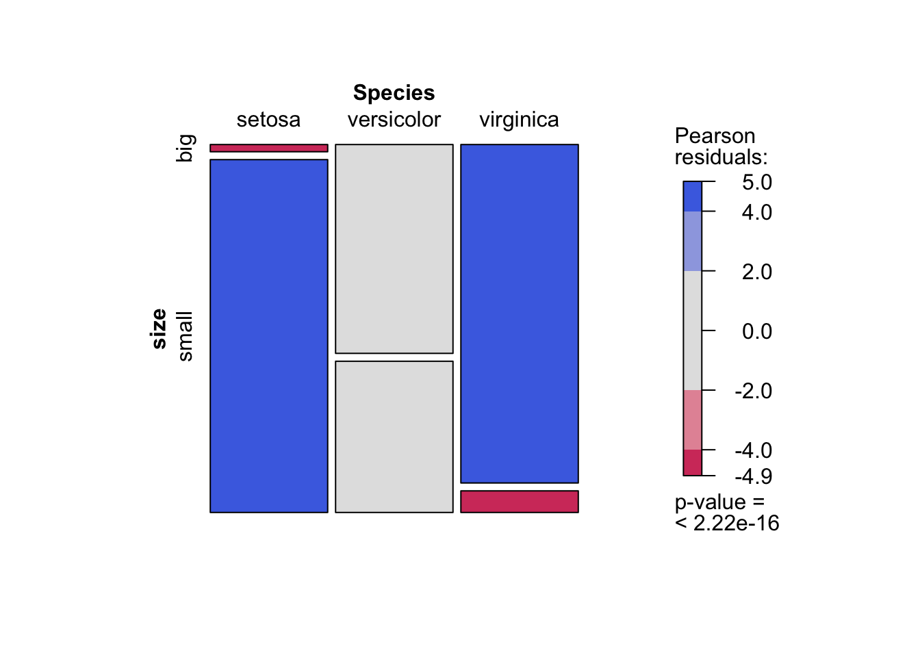
A significant p-value tells us that an association exists, but it doesn't tell us which specific categories are driving that association. Is setosa more likely to be 'small' than expected? Is virginica less likely? This is a form of post-hoc analysis.
Standardized Residuals
The best way to answer this is by examining the standardized residuals. A residual is simply (Observed - Expected). A standardized residual adjusts this value so it follows a standard normal distribution (like a z-score).
The rule of thumb for interpretation is:
- A standardized residual with an absolute value greater than ~2 (more precisely, 1.96) indicates a significant contribution from that cell.
- A positive residual means we observed more cases than expected.
- A negative residual means we observed fewer cases than expected.
The rstatix::chisq_descriptives() function provides a rich table including observed counts, expected counts, and residuals.
chisq_descriptives(test_result)
Look at the std.resid column in the output. For our iris example, you will see large positive and negative residuals, pinpointing exactly which species-size combinations are unusual.
Visualizing Residuals with a Mosaic Plot
A mosaic plot is a fantastic visualization for a contingency table that also shows the residuals. The area of each tile is proportional to the cell's frequency, and the color indicates the standardized residual.
# We need the contingency table object created with base R's table()
contingency_table_base <- table(iris_cat$Species, iris_cat$size)


# Create the mosaic plot
mosaicplot(contingency_table_base, shade = TRUE, main = "Mosaic Plot of Species vs. Size")
4. Quantifying the Strength: Effect Size
Just like in our previous lessons, a significant p-value doesn't tell us about the strength of the association. For a chi-square test, the most common effect size measure is Cramér's V. It ranges from 0 (no association) to 1 (perfect association).
You can calculate it easily with rstatix.
cramer_v(contingency_table_base)
General guidelines for interpreting Cramér's V (the exact values depend on the degrees of freedom, but these are a good start):
- ~0.1: Small effect
- ~0.3: Medium effect
- ~0.5: Large effect
For our iris data, Cramér's V will be quite large, indicating a strong association between species and flower size.
5 Chi-squared Test – Notes on Statistics with R (SwR) - Bookdown
To learn how to dig deeper into a significant result, let's return to this detailed guide.
First, read the section on Standardized residuals. Focus on the introduction, which explains why we need them, and the part that discusses interpretation (values > 1.96). Note the recommendation for rstatix as a good option. Then, read the section on effect sizes to understand Cramér's V and how to interpret its value.
5. Video Summary
To see these steps in action, this short video provides a clear, conceptual walkthrough. While it uses base R's chisq.test() function, the core ideas of creating a table, running the test, and checking assumptions are identical.
Chi-Square Test, Fisher’s Exact Test, & Cross Tabulations in R | R Tutorial 4.10| MarinStatsLectures
This video from MarinStatsLectures quickly covers the main workflow for a Chi-Square test in R.
Watch the introduction on creating a contingency table. See how to create a bar plot to visualize the data. Finally, watch the demonstration of the chi-square test itself, including how to access the expected counts to check assumptions.
Conclusion
You have now added another essential hypothesis test to your analytical toolkit. You can confidently move between comparing means of continuous data (t-tests) and investigating associations in categorical data (chi-square tests), a crucial skill for analyzing diverse datasets in clinical research.
Key Takeaways:
- The chi-square () test of independence is used to determine if there is a statistically significant association between two categorical variables.
- The test's logic is based on comparing observed frequencies with the expected frequencies that would occur if there were no association.
- In R, you can perform the test using
rstatix::chisq_test(variable1 ~ variable2). A p-value < 0.05 indicates a significant association. - After finding a significant association, use standardized residuals (values > |2|) and mosaic plots to identify which specific cells are driving the relationship.
- Use Cramér's V to measure the effect size, or strength, of the association.
Preview of the Next Lesson:
So far, we have compared one mean to a value (one-sample t-test) and the means of two groups (two-sample t-test). But what if your research question involves comparing the means of three or more groups? For example, comparing the effectiveness of Drug A, Drug B, and a Placebo. This requires a new technique. In our next lesson, we will learn about Analysis of Variance (ANOVA) and the post-hoc tests that follow it.