Welcome to the next lesson in our module on regression modeling. In our previous session, you learned how to convert the log-odds from a logistic regression model into interpretable odds ratios. We even had a sneak peek at the broom package, using broom::tidy(exponentiate = TRUE) to streamline that process.
Today, we will dive deep into the broom package and formalize its use in your analysis workflow. This lesson addresses a fundamental challenge in R: the output from statistical models is often complex and inconsistently formatted, making it difficult to use programmatically. You'll learn how broom elegantly solves this by converting model outputs into predictable, "tidy" data frames. We will focus on two essential functions: broom::tidy() for extracting coefficient-level details and broom::glance() for getting a high-level summary of model performance. Mastering broom is a significant step toward the efficient, reproducible, and "industry ready" analysis workflow you're aiming to build.
The Problem: Why We Need broom
When you run a statistical model in R, such as with lm() or glm(), the object that is returned contains a wealth of information. However, accessing this information can be cumbersome. The standard summary() function prints a nice-looking report for a human to read, but it's not a data structure you can easily work with.
Imagine you've fit a simple linear model:
# Fit a linear model predicting miles-per-gallon from weight
car_model <- lm(mpg ~ wt, data = mtcars)


# Look at the standard summary
summary(car_model)
The output shows you the call, residuals, a coefficient table, and overall model statistics like R-squared. Now, what if you wanted to create a plot of the coefficients with their confidence intervals, or compare the R-squared values from ten different models? You would have to manually extract each piece of information, often using awkward code, and then piece it all together into a data frame. This process is tedious and error-prone.
This short video provides an excellent overview of this exact problem and introduces broom as the solution.
Broom: Converting Statistical Models to Tidy Data Frames
This video from Work-Bench, presented by data scientist David Robinson, clearly explains why standard R model outputs are considered "messy" and how they disrupt a tidy analysis workflow.
Watch the first few minutes, from the beginning to the introduction of broom. Pay close attention to the four issues he identifies with the standard summary() output, such as information being stored in row names and inconvenient column names. This perfectly frames the problem broom is designed to solve.
As the video highlights, model objects are messy. They interrupt the "flow" of analysis that you experience when using tidyverse tools like dplyr and ggplot2. broom is the bridge that brings your modeling results back into the tidyverse.
The broom Philosophy: Tidy, Augment, Glance
The broom package provides three core functions, or "verbs," each designed to extract a different kind of information from a model object and turn it into a tidy tibble (a modern data frame).
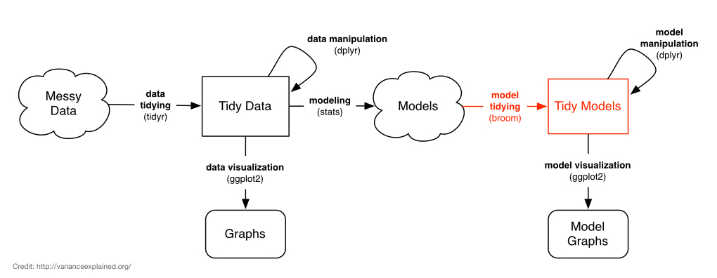
The three main functions are:
tidy(): Summarizes the statistical components of the model on a per-component basis. For a regression model, this means one row for each coefficient (term).glance(): Provides a one-row summary of the entire model. It gives you model-level statistics like R-squared, AIC, and the overall p-value.augment(): Adds model-derived information, like fitted values and residuals, back to the original dataset on a per-observation basis. We won't focus on this function today, but it's good to know it exists.
Let's explore tidy() and glance() in detail. The following reading from the official broom documentation will walk you through these functions with the lm() example we started with.
This vignette is the foundational document for the broom package. It clearly lays out the purpose and usage of its main functions.
Start by reading the section that defines the three tidying functions. Then, follow the example where the author fits a linear model with lm(). Observe the standard summary() output, and then see how broom transforms it. Focus on the sections demonstrating tidy() and glance(). Notice how the output of each function is a clean, well-structured tibble.
Using tidy() to Summarize Model Coefficients
As you saw, tidy() takes the coefficient table from a model summary and turns it into a proper data frame.
library(broom)


# Let's use our car model again
car_model <- lm(mpg ~ wt, data = mtcars)


# Tidy the model object
tidy(car_model)
This produces a tibble like this:
# A tibble: 2 × 5
  term        estimate std.error statistic  p.value
  <chr>          <dbl>     <dbl>     <dbl>    <dbl>
1 (Intercept)    37.3      1.88       19.9   8.24e-19
2 wt             -5.34     0.559      -9.56  1.29e-10
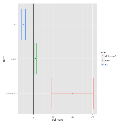
This output is immediately useful. The messy row names are now a proper character column called term, and the column names are clean and predictable. With this data frame, you can now use dplyr to filter for significant terms or ggplot2 to create a coefficient plot.
Using glance() to Summarize Model Fit
While tidy() gives you the details of each component, glance() gives you the big picture. It summarizes the entire model's quality and fit into a single row.
# Glance at our car model
glance(car_model)
The output is a one-row tibble:
# A tibble: 1 × 12
  r.squared adj.r.squared sigma statistic  p.value    df logLik   AIC   BIC deviance df.residual  nobs
      <dbl>         <dbl> <dbl>     <dbl>    <dbl> <dbl>  <dbl> <dbl> <dbl>    <dbl>       <int> <int>
1     0.753         0.745  3.05      91.4 1.29e-10     1  -80.0  166.  170.     278.          30    32
This is incredibly powerful. All the key metrics you need to evaluate the model—r.squared, adj.r.squared, AIC, BIC, and the model's overall p.value—are neatly organized. The true power of glance() becomes apparent when you have many models and want to compare them, a topic we'll explore in the next lesson.
The following reading provides more practical examples in a medical research context, showing how tidy() and glance() are used in a typical tidyverse pipeline.
Chapter 32 Linear Regression and Broom for Tidying Models | Reproducible Medical Research with R
This chapter from "Reproducible Medical Research with R" demonstrates the complete workflow of building a model and then immediately using broom functions to inspect the results.
First, read the section that builds a simple null model and introduces tidy() and glance(). Then, see how glance() is used to compare the fit of the null model to a model with predictors in the next section. Finally, read the section on interpreting the tidy output, which breaks down what each column from tidy() means. This connects the abstract concept of a tidy output to the practical task of interpreting your model's coefficients.
An Advanced Workflow: Combining broom with purrr
To give you a glimpse of the "extravagant build" you're interested in, consider a common task in research: running the same analysis on different subgroups of your data. For example, fitting a separate regression model for each drug treatment group or for each hospital in a multi-center study.
Manually, this would be a nightmare. But by combining dplyr::group_by(), purrr::map(), and broom::glance(), you can perform this complex analysis in a few lines of code, yielding a clean, comparable table of results. The following video demonstrates this powerful pattern.
Multiple Linear Regressions in R (Bonus: Summary Table)
In this video, Matt Dancho of Business Science demonstrates a powerful workflow for performing grouped regressions.
Watch the section from this clip. He takes a dataset, splits it into groups, runs a linear regression on each group, and then uses broom::glance() combined with map_dfr() to collect all the model summaries into a single, tidy data frame. You don't need to memorize the code right now, but focus on understanding the workflow and the power that broom unlocks.
This approach—grouping, modeling, and tidying—is a cornerstone of modern, scalable data analysis in R. It allows you to move from analyzing one model to analyzing hundreds with minimal extra effort.
Conclusion
In this lesson, you have moved beyond using broom for a single, specific task and have learned its general-purpose role in a modern R workflow. You now understand how to systematically convert messy model outputs into clean, usable data frames.
Key Takeaways:
- Standard R model objects produce outputs that are difficult to work with programmatically.
- The
broompackage solves this by providing consistent functions to "tidy" model objects. broom::tidy()creates a tibble with one row for each component of the model, such as a coefficient. It's ideal for analyzing and visualizing individual term estimates.broom::glance()creates a one-row tibble summarizing the entire model's fit and quality. It's perfect for comparing multiple models.- By making model outputs tidy,
broomallows you to seamlessly integrate your modeling results withtidyversetools likedplyrandggplot2.
Preview of the Next Lesson:
We've now seen that glance() gives us powerful model comparison metrics like AIC (Akaike's Information Criterion) and BIC (Bayesian Information Criterion). In our next lesson, we will focus on the art and science of model comparison. You will learn how to use these metrics, along with statistical tests like the analysis of variance (anova()), to formally compare different models and select the one that best explains your data while avoiding overfitting.