Bayes' Rule for Robot State Estimation

Welcome to your fourth lesson. In our previous session, we established a crucial mathematical tool: the Jacobian matrix. You learned how it provides a local linear approximation for non-linear functions, which is essential for propagating Gaussian uncertainty through realistic robot models and for understanding the kinematics of robotic arms.

So far, we have the components to describe a robot's state and its uncertainty. However, we are missing the central mechanism that allows a robot to learn from its senses. How does a robot refine its belief about where it is when it receives a new, noisy sensor reading? This lesson introduces the theoretical foundation for answering that question: Bayes' Rule. You will see how this single, elegant rule of probability provides the recipe for all probabilistic state estimation in robotics, forming the core logic of what is known as the Bayes Filter.

By the end of this lesson, you will be able to explain how Bayes' Rule is used to formally update a robot's belief about its state in a recursive cycle of prediction and correction, based on its actions and observations.

1. The Core Problem: Causal vs. Diagnostic Reasoning

At the heart of state estimation is a fundamental challenge. It is often straightforward to model how a sensor will behave given a known state, but what we actually want is the reverse: to deduce the state given a sensor reading. This is the difference between causal and diagnostic reasoning.

Causal Knowledge: Knowing the state, what is the probability of a certain measurement? For example: "If I am directly in front of a door, my sensor has a 90% chance of reporting 'door'." This is the sensor model, written as $P (measurement ∣ state)$ . It is relatively easy to determine by testing the sensor.
Diagnostic Knowledge: Having received a measurement, what is the probability that I am in a certain state? For example: "My sensor reported 'door'. What is the probability that I am actually in front of a door?" This is what the robot needs to figure out, written as $P (state ∣ measurement)$ .

Bayes' Rule provides the mathematical bridge to get from the causal knowledge we can easily model to the diagnostic knowledge we need.

The Bayes Filter for Robotic State Estimation - Russ Stuff

This article provides an excellent introduction to this distinction. The author uses a simple weather station example to make the concept clear before applying it to robotics.

Read the section titled "Causal vs Diagnostic Reasoning". Pay close attention to how Bayes' Rule is used to convert the easily obtained causal probabilities (e.g., the sensor's accuracy) into the desired diagnostic probability (the chance of rain given a 'wet' reading).

2. Bayes' Rule in Robotics

Let's formalize this for a robot. We represent the robot's knowledge about its own state as a probability distribution called a belief. Bayes' Rule tells us how to update this belief when we get a new measurement, $z$ .

The rule is:

P (x ∣ z) = \frac{P ( z ∣ x ) P ( x )}{P ( z )}

Let's break this down into the standard robotics terminology:

$P (x ∣ z)$ is the Posterior. This is our updated belief about the state $x$ after incorporating the measurement $z$ . This is what we want to compute.
$P (z ∣ x)$ is the Likelihood. This is the Sensor Model (or Measurement Model). It's the causal knowledge we discussed: the probability of getting measurement $z$ given that the robot is in state $x$ .
$P (x)$ is the Prior. This is our belief about the state $x$ before the measurement.
$P (z)$ is the Evidence (or Marginal Likelihood). It's the total probability of observing measurement $z$ . In practice, this term can be difficult to compute. Luckily, it doesn't depend on the state $x$ , so we can treat it as a normalization constant, often denoted $η$ , that ensures our posterior probabilities sum to 1.

This gives us the practical form of the rule for a single update:

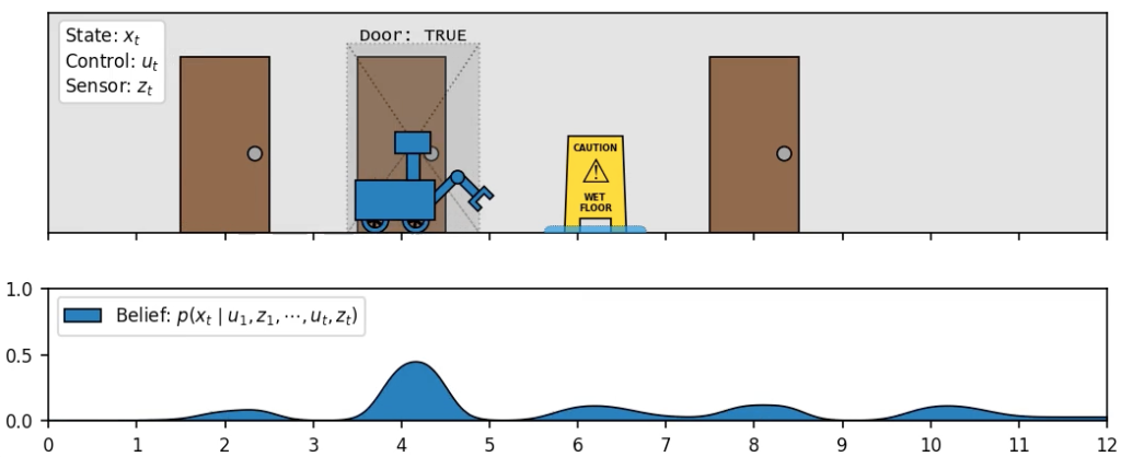
Posterior = η \cdot Likelihood \cdot Prior

b e l (x) = η \cdot P (z ∣ x) \cdot b e l (x)

Imagine a robot in a 1D hallway. Initially, it has no idea where it is, so its belief (the prior) is a uniform distribution across the entire hallway. Then, its sensor reports "door: TRUE". We use our sensor model (the likelihood) to update the belief. The new belief (the posterior) will have high probabilities at the locations of the doors and low probabilities everywhere else.

A robot in a 1D hallway receives a sensor reading that it is near a door. Its initial, less certain belief (not shown) is updated using the sensor model. The resulting posterior belief, shown in the lower plot, is a multi-modal distribution with peaks corresponding to the known door locations. The highest peak reflects the robot's best current guess.

3. The Bayes Filter: Recursive State Estimation

A robot doesn't just make one measurement. It is in a constant loop of acting and sensing. We need a way to apply Bayes' rule recursively over time. This process is called the Bayes Filter. It consists of a two-step cycle that repeats for each time step: Prediction and Correction.

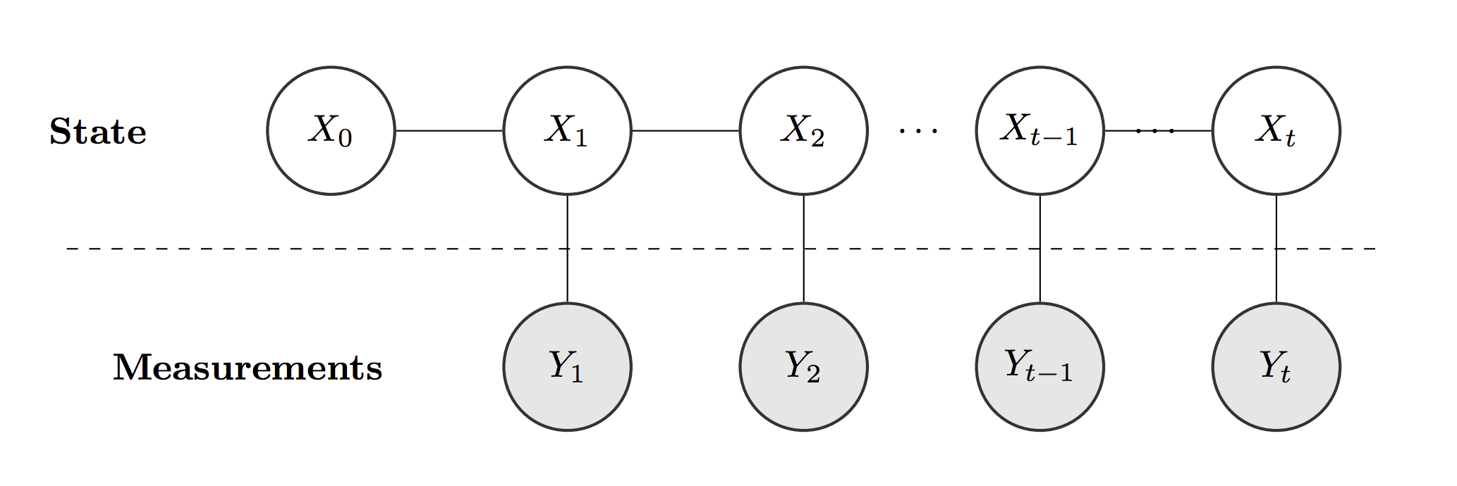
This diagram shows the structure of a Hidden Markov Model (HMM), which is the graphical representation of the assumptions in a Bayes filter. The state $X_t$ is 'hidden' and only depends on the previous state $X_{t-1}$ and an action (not shown). The measurement $Y_t$ is 'observed' and only depends on the current state $X_t$.

The key insight is that our belief from the end of the last time step, $b e l (x_{t - 1})$ , becomes the foundation for the belief at the current time step, $b e l (x_{t})$ .

Step 1: Prediction (The Action Update)

First, the robot acts. It executes a control command $u_{t}$ (e.g., "drive forward 1 meter"). This action is never perfect; there's always noise (e.g., wheels slipping). We use a Motion Model $P (x_{t} ∣ u_{t}, x_{t - 1})$ to predict the new state distribution. This step propagates our previous belief $b e l (x_{t - 1})$ forward in time, incorporating the uncertainty from the action. This generally "smears out" or increases the uncertainty in our belief.

The result is the predicted belief, or the new prior, which we denote $b e l (x_{t})$ .

b e l (x_{t}) = \int P (x_{t} ∣ u_{t}, x_{t - 1}) b e l (x_{t - 1}) d x_{t - 1}

This integral sums up the probabilities of arriving at state $x_{t}$ from all possible previous states $x_{t - 1}$ , weighted by the belief we had in those previous states.

Step 2: Correction (The Measurement Update)

Next, the robot senses. It gets a new measurement $z_{t}$ . This is exactly the single update step we saw before. We use the Sensor Model $P (z_{t} ∣ x_{t})$ to correct our predicted belief $b e l (x_{t})$ . This step incorporates the new information and typically "sharpens" our belief, reducing uncertainty.

The result is the new posterior belief, $b e l (x_{t})$ .

b e l (x_{t}) = η P (z_{t} ∣ x_{t}) b e l (x_{t})

This two-step cycle, Predict then Correct, is the essence of the Bayes filter. The posterior belief at the end of one time step, $b e l (x_{t})$ , becomes the input prior for the prediction step of the next time step, $b e l ((x_{t + 1} - 1))$ .

4. Deriving the Bayes Filter

To give you the "rock solid" foundation you appreciate, let's walk through how these equations are formally derived. The derivation relies heavily on the laws of probability and the Markov Assumption, which states that the current state is a "complete" summary of the past.

Bayes Filter (Cyrill Stachniss)

The video "Bayes Filter" by Cyrill Stachniss, a leading robotics educator, provides one of the clearest derivations of this framework. We will walk through the key parts of his derivation.

Please watch the following segments: Introduction and Example (watch this segment): The video begins by defining recursive state estimation and uses the same 1D hallway example to build your intuition about how belief evolves through prediction (smearing) and correction (sharpening). The Derivation (watch this segment): This is the core of the lesson. The presenter derives the Bayes filter equation from first principles. As you watch, focus on identifying these key steps: Applying Bayes' Rule to swap the current state x_t and measurement z_t. Applying the Markov Assumption to simplify the measurement likelihood term P(z_t | \dots) to just P(z_t|x_t). Using the Law of Total Probability to introduce the previous state x_{t-1} into the equation, which is the key to making it recursive. Applying the Markov Assumption again, this time to simplify the motion term P(x_t | \dots) to just P(x_t | x_{t-1}, u_t). Recognizing that the final term is simply the belief from the previous time step, bel(x_{t-1}). Prediction and Correction (watch this segment): Finally, the presenter re-organizes the final equation into the distinct prediction and correction steps that form the algorithm's structure. He explicitly defines the Motion Model and Observation (Sensor) Model.

The final equation derived in the video combines these steps:

b e l (x_{t}) = η Sensor Model P (z_{t} ∣ x_{t}) \int Motion Model P (x_{t} ∣ u_{t}, x_{t - 1}) Old Belief b e l (x_{t - 1}) d x_{t - 1}

This single equation elegantly captures the entire recursive process of a robot updating its understanding of the world.

Conclusion

In this lesson, we moved from individual mathematical tools to the core philosophical and algorithmic framework for probabilistic robotics. You now understand how a robot can rigorously reason about its own state in the presence of uncertainty.

Key Takeaways:

Bayes' Rule is the fundamental engine that allows a robot to update its belief, turning easily-modeled causal knowledge ( $P (measurement ∣ state)$ ) into the diagnostic knowledge it needs ( $P (state ∣ measurement)$ ).
The Bayes Filter is a recursive, two-step algorithm that applies this logic over time.
1. Predict: Use a Motion Model to project the belief forward, incorporating uncertainty from actions.
2. Correct: Use a Sensor Model and the latest measurement to refine the predicted belief.
The entire framework rests on the Markov Assumption, which states that the present state contains all the information needed to predict the future, making the recursive updates possible.
The Bayes Filter is a framework, not a single algorithm. How we represent the belief (e.g., histograms, Gaussians, particles) leads to different specific filter implementations like the Kalman Filter or Particle Filter, which we will encounter later.

You have now completed the core theoretical foundations of this module. In our next lesson, we will make these concepts concrete. You will implement your first filter from scratch: a discrete Bayes filter in Python to solve the 1D hallway localization problem we've been using as our example.

Recommended resources