Visualizing Meal Quality Trends Over Time

Preparing Your Data for Time Series Analysis

Before we can analyze trends, your data must be structured correctly. For time series analysis in pandas, this means ensuring dates are represented not as simple strings, but as datetime objects. The most effective way to work with this data is to set the datetime column as the DataFrame's index, creating a DatetimeIndex. This unlocks a powerful suite of time-based indexing and analysis tools.

Let's assume your data, after processing and model predictions, is in a pandas DataFrame with columns like date, quality_score, and violation_count. The first step is to correctly parse the date column.

The following video from Corey Schafer provides a clear, practical guide on how to convert string columns to datetime objects and set them as an index.

Once your DataFrame has a DatetimeIndex, you can easily extract time-based features like the month or day of the week, which will be essential for analyzing seasonality. The "Time Series Analysis with Pandas" tutorial provides an excellent overview of this process.

Your initial code to prepare your DataFrame, which we'll call df, would look something like this:

import pandas as pd




# Assume 'df' is your DataFrame
# Convert the 'date' column to datetime objects
df['date'] = pd.to_datetime(df['date'])




# Set the 'date' column as the index
df.set_index('date', inplace=True)




# Create columns for easier grouping later
df['month'] = df.index.month
df['day_of_week'] = df.index.day_name()




# Sort the index to ensure chronological order for plotting
df.sort_index(inplace=True)

Visualizing and Aggregating Trends Over Time

With your data prepared, you can start exploring. The most straightforward approach is to plot your metrics over time. However, daily data can be very "noisy," making it difficult to see underlying patterns. Two key techniques help us manage this: resampling and rolling windows.

Resampling

Resampling changes the frequency of your time series. For your project, you'll likely downsample your daily data into weekly or monthly aggregates. This involves grouping data points into time bins (e.g., all days in a week) and applying an aggregation function like .mean(), .sum(), or .count(). This is perfect for calculating the average weekly quality score or the total number of violations per month.

The Dataquest tutorial provides a clear explanation of how to use the .resample() method.

If you need to apply different aggregations to different columns simultaneously (e.g., mean of quality_score but sum of violation_count), the .agg() method is extremely useful.

Rolling Windows

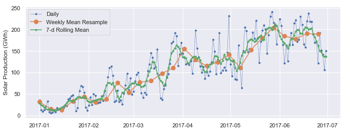
A rolling window calculates an aggregate over a sliding window of a fixed size (e.g., a 7-day rolling average). Unlike resampling, it maintains the original frequency of the data but produces a smoothed version. This is excellent for visualizing a trend line that isn't as jagged as the raw data.

The following image and reading illustrate the difference between resampling and a rolling mean.

Analyzing Seasonality with Plots

Now you can use these techniques to create plots that directly address your project's questions about seasonality.

Box Plots for Monthly and Weekly Patterns

To check for a drop in quality during the monsoon season (roughly June-September in many parts of India), you can group your data by month and create box plots. This will show the distribution of quality scores for each month, making it easy to spot if certain months have consistently lower scores. Similarly, grouping by day of the week can reveal any weekly patterns.

Seasonal Decomposition

A more formal way to analyze temporal patterns is seasonal decomposition, which separates a time series into three components:

1. Trend: The long-term progression of the series (e.g., is meal quality generally improving over the years?).
2. Seasonality: The repeating, periodic patterns (e.g., yearly monsoon effect, weekly cycles).
3. Residual: The leftover "noise" after removing the trend and seasonality.

This video provides an excellent conceptual overview.

The statsmodels library makes it incredibly easy to perform this decomposition. The resulting plots provide a powerful summary of your data's temporal structure.

The GeeksforGeeks article provides the code to generate such a plot.

Conclusion

In this lesson, you've learned the fundamental techniques for temporal analysis in pandas. You can now take your time-stamped data and transform it into insightful visualizations that reveal underlying trends and patterns.

Here are the key takeaways:

• Data Preparation is Key: Always convert date columns to a datetime type and set them as the DataFrame index for effective analysis.
• Aggregate to See the Big Picture: Use .resample() to group your data into daily, weekly, or monthly buckets to calculate aggregate metrics like mean quality or total violations.
• Smooth to Find the Trend: Use .rolling() to compute moving averages, which smooths out noise and helps visualize the underlying trend.
• Visualize Seasonality: Use line plots of resampled data and box plots grouped by month or day of the week to identify recurring patterns like monsoon effects or weekly cycles.
• Decomposition Provides Structure: Use statsmodels.tsa.seasonal_decompose to formally separate your time series into trend, seasonal, and residual components for a comprehensive overview.

You now have the tools to complete the temporal analysis portion of your project. In the next lesson, we will build on this by using statistical tests, such as the chi-square test, to quantify the strength of the relationship between categorical variables, like school type and violation presence.