Evaluating Image Classifier Performance

1. Beyond Accuracy: A Framework for Evaluation

When dealing with imbalanced data, your primary goal isn't just to be correct most of the time; it's to be correct about the things that matter most. For your project, failing to identify a 'Poor' quality meal (a false negative) is a far more severe error than misclassifying an 'Adequate' meal as 'Poor' (a false positive). The evaluation metrics we'll cover help you quantify this distinction.

The flowchart below provides an excellent mental model for choosing the right metric based on your project's needs.

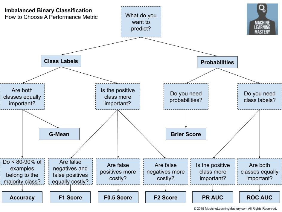
This flowchart guides you through selecting an appropriate performance metric for imbalanced classification tasks based on what you want to predict and what errors are more costly.

Since you are predicting class labels ('Good', 'Adequate', 'Poor') and are particularly concerned about missing violations, you'll be focusing on the branch where the positive class ('Poor') is more important and false negatives are costly. This leads us to metrics like Recall and the F-beta scores.

2. The Confusion Matrix: Deconstructing Predictions

The foundation of all classification metrics is the confusion matrix. It's a simple table that breaks down your model's performance by comparing its predictions to the actual ground truth labels. For a binary problem (e.g., 'Poor' vs. 'Not Poor'), it has four cells:

• True Positives (TP): The model correctly predicted the positive class. (It said 'Poor', and it was 'Poor').
• True Negatives (TN): The model correctly predicted the negative class. (It said 'Not Poor', and it was 'Not Poor').
• False Positives (FP): The model incorrectly predicted the positive class. (It said 'Poor', but it was 'Not Poor'). This is a "false alarm."
• False Negatives (FN): The model incorrectly predicted the negative class. (It said 'Not Poor', but it was 'Poor'). This is a "missed detection" and the most critical error type for your project.

The StatQuest video below gives an excellent, intuitive explanation of how to build and read a confusion matrix.

3. Precision vs. Recall: A Critical Trade-off

Once you have the values from the confusion matrix, you can calculate more insightful metrics. The two most important are Precision and Recall.

This diagram visually contrasts how Precision and Recall are calculated from the confusion matrix. Precision focuses on the set of positive predictions, while Recall focuses on the set of actual positive instances.

Precision

Precision answers the question: "Of all the instances the model predicted as positive, what fraction was actually positive?"

In your project's context, high precision means that when your model flags a meal as 'Poor', it's very likely to be correct. This reduces the number of false alarms.

Recall (or Sensitivity)

Recall answers the question: "Of all the actual positive instances, what fraction did the model successfully identify?"

For your Midday Meal project, high recall is paramount. It means your model is effective at finding most of the 'Poor' quality meals, minimizing the dangerous false negatives.

There is often a trade-off between precision and recall. A model tuned to be extremely sensitive (high recall) might generate more false positives, lowering its precision. Your goal is to find a balance that meets your project's needs.

F1-Score

The F1-score is the harmonic mean of precision and recall. It provides a single score that balances both metrics, making it a useful overall measure, especially when you have an imbalanced class distribution.

The F1-score is a good target for your baseline model, as specified in your project plan (F1 > 0.70). It ensures that your model is not only finding the violations (high recall) but also being reasonably accurate when it does so (decent precision).

The following video provides a fantastic walkthrough of these concepts and then shows how to calculate them in Python.

4. Implementation: Evaluating Your PyTorch Model

Now, let's bring these concepts into your code. While you could calculate these metrics manually, the scikit-learn library provides robust and easy-to-use functions. The process involves two main steps:

1. Get Predictions: Run your trained model on the validation or test dataset to get its output predictions.
2. Calculate Metrics: Use sklearn.metrics functions with the model's predictions and the true labels to generate the confusion matrix and a full classification report.

First, you need a function to get all predictions and labels from a dataloader. This function should set the model to evaluation mode (model.eval()) and use torch.no_grad() to disable gradient calculations, which speeds up inference.

import torch
import numpy as np
from sklearn.metrics import classification_report, confusion_matrix

def get_all_preds(model, dataloader, device):
    all_preds = torch.tensor([]).to(device)
    all_labels = torch.tensor([]).to(device)
    model.eval() # Set model to evaluation mode
    with torch.no_grad():
        for images, labels in dataloader:
            images = images.to(device)
            labels = labels.to(device)
            
            outputs = model(images)
            # Get the predicted class with the highest probability
            _, preds = torch.max(outputs, 1)
            
            all_preds = torch.cat((all_preds, preds), dim=0)
            all_labels = torch.cat((all_labels, labels), dim=0)

    return all_preds.cpu().numpy(), all_labels.cpu().numpy()

# After your training loop finishes...
# device = torch.device("cuda" if torch.cuda.is_available() else "cpu")
# model = your_trained_model
# val_loader = your_validation_dataloader

# Get predictions and true labels
y_preds, y_true = get_all_preds(model, val_loader, device)

# Now, use scikit-learn to evaluate
print("Confusion Matrix:")
print(confusion_matrix(y_true, y_preds))

print("\nClassification Report:")
# Assuming your classes are 'Good', 'Adequate', 'Poor' mapped to 0, 1, 2
target_names = ['Good', 'Adequate', 'Poor'] 
print(classification_report(y_true, y_preds, target_names=target_names))

This classification_report is extremely powerful. It gives you the precision, recall, and F1-score for each class individually, as well as averaged scores. For your project, you'll want to pay close attention to the row corresponding to the 'Poor' class.

The following article demonstrates a similar process, integrating sklearn.metrics to evaluate a model at the end of a PyTorch workflow.

If you want to see how precision and recall can be calculated from scratch within a PyTorch training loop, you can refer back to the Paperspace article from our last lesson.

Conclusion

You are now equipped with the essential tools to rigorously evaluate your image classification model. You've moved beyond simple accuracy to a more nuanced understanding of model performance that is directly aligned with your project's objectives.

Here are the key takeaways from this lesson:

• A confusion matrix is the starting point for evaluation, breaking down predictions into True/False Positives and Negatives.
• Precision measures the reliability of your model's positive predictions (how many flagged meals are actually 'Poor').
• Recall measures the model's ability to find all positive instances (how many of the actual 'Poor' meals did it find). For your project, this is arguably the most critical metric.
• The F1-score provides a balanced summary of precision and recall, serving as an excellent target metric for overall performance.
• scikit-learn's classification_report and confusion_matrix are the standard, practical tools for implementing this evaluation in your Python code.

With your first baseline model trained and properly evaluated, you are ready to tackle the next modality. In the upcoming lesson, we will build your second baseline: a text-only classifier for parent complaints. You'll be introduced to the powerful Transformer architecture and learn how to fine-tune a state-of-the-art model like BERT for your specific task.