PyTorch Fusion Model for Violation Severity Prediction

The Fusion Model Architecture

Before we write code, let's visualize the model we're about to build. At this stage, your fine-tuned ResNet and BERT models act as fixed feature extractors. We will no longer train them. Instead, we feed them data in evaluation mode (.eval()) to generate high-level feature vectors. Our new fusion model is a separate, smaller network that learns how to interpret the combination of these features.

This new model will take three inputs:

1. The image feature vector from ResNet.
2. The text feature vector (CLS token embedding) from BERT.
3. The numerically encoded metadata vector (school type, season, etc.).

It will then concatenate these vectors into a single, long vector and pass it through a simple classifier—a Multi-Layer Perceptron (MLP)—to make the final prediction.

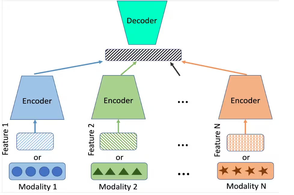
The structure of the MLP itself is quite standard. It combines different types of features, much like how you might process separate categorical and continuous data streams before feeding them into a final prediction layer.

Building the Fusion Model in PyTorch

The most elegant way to implement this in PyTorch is by creating a custom class that inherits from torch.nn.Module. This class will define the layers of our fusion MLP and specify how data flows through them in the forward method.

The key operation will be torch.cat(), which concatenates a sequence of tensors along a given dimension. This is how we'll merge the feature vectors from our different modalities.

Inspired by that video, let's outline the structure of your FusionModel.

1. Defining the FusionModel Class

Your model's __init__ method will define the layers of the MLP. You need to know the size of the input feature vectors to calculate the input dimension for your first linear layer.

• Image Features: Your fine-tuned ResNet model likely produces a vector of size 2048 (if using the standard ResNet-50).
• Text Features: A base BERT model produces a [CLS] token embedding of size 768.
• Metadata Features: The size of this vector depends on your encoding scheme (e.g., number of categories in one-hot encoding). Let's assume it's 10 for this example.

The total input dimension for your MLP will be the sum: $2048+768+10=2826$.

Your forward method will accept the three feature tensors, concatenate them, and pass them through the MLP layers. Here is a Python-like pseudocode structure for your class:

import torch
import torch.nn as nn

class FusionModel(nn.Module):
    def __init__(self, num_image_features, num_text_features, num_meta_features, num_classes, hidden_size=512):
        super().__init__()
        



        # Calculate the total input size after concatenation
        total_input_features = num_image_features + num_text_features + num_meta_features
        



        # Define the fusion MLP
        self.fusion_layer = nn.Sequential(
            nn.Linear(total_input_features, hidden_size),
            nn.ReLU(),
            nn.Dropout(0.3),
            nn.Linear(hidden_size, num_classes)
        )

    def forward(self, image_features, text_features, metadata_features):



        # Concatenate features along the feature dimension (dim=1)
        # Assumes batch dimension is dim=0
        fused_features = torch.cat([image_features, text_features, metadata_features], dim=1)
        



        # Pass the concatenated vector through the fusion MLP
        output = self.fusion_layer(fused_features)
        
        return output

The Lightly.ai article below also provides a concrete code example that, while labeled "Early Fusion," demonstrates the exact torch.cat mechanism we're using to combine pre-extracted feature vectors.

Data Pipeline for the Fusion Model

Running the large ResNet and BERT models for every training step of our small fusion MLP would be incredibly inefficient. A much better approach is to pre-compute the feature vectors.

Your workflow should be:

1. Set your trained ResNet and BERT models to evaluation mode (model.eval()) and disable gradient calculations (with torch.no_grad():).
2. Iterate through your entire dataset (train, validation, and test splits).
3. For each sample, pass the image through ResNet and the text through BERT to get the corresponding feature vectors.
4. Save these feature vectors to disk, along with their corresponding metadata and labels. A good way to organize this is to save a dictionary ({'image_feat': ..., 'text_feat': ..., 'meta_feat': ..., 'label': ...}) for each sample using torch.save().
5. Create a new torch.utils.data.Dataset class, let's call it FusionDataset, that simply loads these pre-computed files in its __getitem__ method.

This way, training your fusion model becomes very fast, as the DataLoader will only be loading small, pre-processed tensors from disk instead of running massive neural networks.

The Training Loop

The training loop for the fusion model follows the standard PyTorch pattern you've implemented before. The main difference is that in each iteration, you will be loading a batch of three feature tensors and one label tensor from your FusionDataLoader.

Here's a summary of the steps inside the loop:

1. Get a batch of data: image_features, text_features, metadata_features, and labels.
2. Move all tensors to the correct device (GPU).
3. Clear the gradients: optimizer.zero_grad().
4. Perform the forward pass: outputs = model(image_features, text_features, metadata_features).
5. Calculate the loss (e.g., using nn.CrossEntropyLoss): loss = criterion(outputs, labels).
6. Perform the backward pass: loss.backward().
7. Update the model's weights: optimizer.step().

You can refer back to the detailed training loop implementation in the BERT fine-tuning tutorial you used previously as a robust template.

Conclusion

In this lesson, you have learned the practical steps to build and train a late fusion model in PyTorch. This is a major milestone in your project, marking the point where individual components are integrated into a cohesive, multimodal system.

The key takeaways are:

• Model Implementation: A fusion model can be defined as a custom nn.Module class containing a simple MLP to process concatenated features.
• Feature Concatenation: The torch.cat() function is the core mechanism for merging feature vectors from different modalities.
• Efficient Data Handling: Pre-computing and saving feature vectors from your large models is a critical optimization that makes training the final fusion classifier fast and efficient.
• Standard Training: The training loop follows the same fundamental PyTorch pattern of forward pass, loss calculation, backpropagation, and optimization.

In our next lesson, we will complete this module by evaluating your newly trained fusion model. You will compare the multimodal model's performance against the single-modality baselines to quantify the benefit of fusion. This will be the moment of truth, where you see if combining image, text, and metadata truly leads to a better violation detection system.