Outputting Key Model Artifacts

From Predictions to Insights

Before we can create any artifacts, we first need a set of predictions. The initial step, which you will perform on your own, is to loop through your test dataset (containing images, text, and metadata), run each data point through the ViolationPredictor class you built, and store the model's output alongside the true labels. This will give you a pandas DataFrame containing y_true (the actual labels) and y_pred (your model's predictions), as well as the associated location and date for each entry.

Once you have this DataFrame, you are ready to generate the following artifacts.

1. The Model Performance Summary

A robust evaluation goes far beyond a single accuracy score. For your project, where identifying 'Poor' quality meals is more critical than correctly classifying 'Good' ones, we need nuanced metrics like precision and recall. A classification report and a confusion matrix provide this detailed view.

The Classification Report

The classification report, generated by scikit-learn, breaks down performance for each class. This is crucial for understanding how well your model identifies different levels of meal quality, especially if your dataset is imbalanced (i.e., has many more 'Good' examples than 'Poor' ones).

The video below offers an excellent explanation of each component in a classification report and highlights why accuracy alone can be misleading.

The Confusion Matrix

While the classification report provides the numbers, a confusion matrix visualizes them, showing exactly where your model is "confused." For example, is it misclassifying 'Adequate' meals as 'Poor', or vice-versa? A heatmap-style confusion matrix makes these patterns immediately obvious.

Implementation

After running your predictions, you'll have lists or pandas Series for y_true and y_pred. You can then generate and save your performance summary with the following code.

import pandas as pd
import seaborn as sns
import matplotlib.pyplot as plt
from sklearn.metrics import classification_report, confusion_matrix




# Assuming 'results_df' is your DataFrame with true labels and predictions
y_true = results_df['true_label']
y_pred = results_df['predicted_label']
class_names = ['Poor', 'Adequate', 'Good'] # Or your specific class labels




# 1. Generate and print the classification report
report = classification_report(y_true, y_pred, target_names=class_names)
print(report)




# Optionally, save the report to a text file
with open('artifacts/classification_report.txt', 'w') as f:
    f.write(report)




# 2. Generate and save the confusion matrix plot
cm = confusion_matrix(y_true, y_pred)
plt.figure(figsize=(8, 6))
sns.heatmap(cm, annot=True, fmt='d', cmap='Blues', 
            xticklabels=class_names, yticklabels=class_names)
plt.xlabel('Predicted Label')
plt.ylabel('True Label')
plt.title('Confusion Matrix for Meal Quality')




# Save the plot to a file
plt.savefig('artifacts/confusion_matrix.png')
print("Confusion matrix saved to artifacts/confusion_matrix.png")

2. The Geospatial Hotspot Map

Your project aims to identify geographic "hotspots" of meal quality violations. Simply plotting the average violation rate per district on a map (a choropleth) is a good start, but it doesn't tell you if a high-violation district is a random outlier or part of a statistically significant cluster.

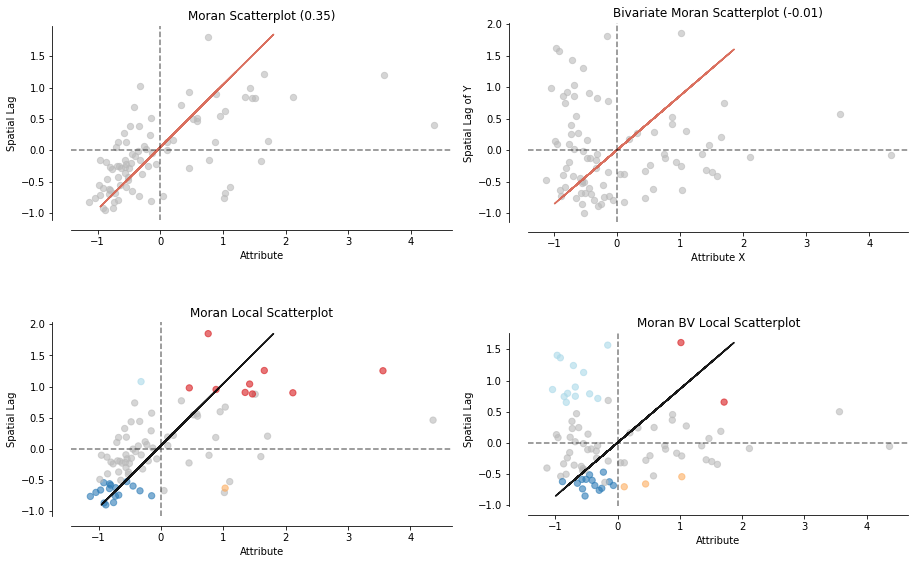
To do this rigorously, we use a technique called Local Indicators of Spatial Association (LISA). LISA analysis helps identify:

• Hotspots (High-High): Districts with high violation rates surrounded by other districts with high violation rates.
• Coldspots (Low-Low): Districts with low violation rates surrounded by others with low rates.
• Spatial Outliers (High-Low, Low-High): A high-violation district surrounded by low-violation ones, or vice-versa.

The following guide from a Geographic Data Science course provides a comprehensive, hands-on walkthrough of this entire process. Since geospatial analysis is new to you, we will follow it closely.

Implementation

Your implementation will adapt the code from the tutorial. You will first need to aggregate your prediction results to get a single violation score per geographic unit (e.g., district). Then, you merge this data with a GeoDataFrame loaded from a shapefile of Indian districts.

import geopandas as gpd
from pysal.lib import weights
from pysal.explore import esda
import matplotlib.pyplot as plt




# 1. Load shapefile and merge with your violation data
#    (Assuming 'district_violations' is a DataFrame with 'district_name' and 'violation_rate')
india_districts = gpd.read_file('path/to/india_districts.shp')
geo_violations = india_districts.merge(district_violations, on='district_name')




# 2. Create spatial weights matrix (Queen contiguity)
#    (Handle islands/unconnected regions as shown in the tutorial)
w = weights.Queen.from_dataframe(geo_violations)
w.transform = 'R' # Row-standardize




# 3. Calculate Local Moran's I (LISA)
lisa = esda.Moran_Local(geo_violations['violation_rate'], w)




# 4. Add LISA results to the GeoDataFrame
geo_violations['significant'] = lisa.p_sim < 0.05
geo_violations['quadrant'] = lisa.q




# 5. Create and save the LISA cluster map
#    (Using the custom plotting code from the tutorial)
fig, ax = plt.subplots(1, figsize=(10, 10))




# Plot non-significant areas
geo_violations[geo_violations['significant'] == False].plot(ax=ax, color='lightgrey')



# Plot HH clusters (hotspots)
geo_violations[(geo_violations['significant'] == True) & (geo_violations['quadrant'] == 1)].plot(ax=ax, color='red')



# Plot LL clusters (coldspots)
geo_violations[(geo_violations['significant'] == True) & (geo_violations['quadrant'] == 3)].plot(ax=ax, color='blue')



# Plot spatial outliers if desired

ax.set_axis_off()
plt.title('Violation Hotspots for Midday Meals', fontsize=16)
plt.savefig('artifacts/hotspot_map.png', dpi=300)
print("Hotspot map saved to artifacts/hotspot_map.png")

3. The Temporal Trend Plot

Finally, you need to investigate temporal patterns. Does meal quality dip during certain times of the year, like the monsoon season, or around festivals? A simple line plot can reveal these trends. This task relies on your existing skills with pandas and matplotlib.

Implementation

You will use your results DataFrame, which should contain a date column for each data point.

import pandas as pd
import matplotlib.pyplot as plt




# Assuming 'results_df' has 'date' and 'violation_score' columns
# (violation_score could be 1 for 'Poor', 0 otherwise)




# 1. Ensure 'date' column is in datetime format
results_df['date'] = pd.to_datetime(results_df['date'])




# 2. Set date as the index to perform time-series operations
time_df = results_df.set_index('date')




# 3. Resample the data by month and calculate the mean violation rate
monthly_violations = time_df['violation_score'].resample('M').mean()




# 4. Create and save the plot
plt.figure(figsize=(12, 6))
monthly_violations.plot(marker='o', linestyle='-')

plt.title('Monthly Average Meal Violation Rate')
plt.xlabel('Date')
plt.ylabel('Average Violation Rate')
plt.grid(True, which='both', linestyle='--', linewidth=0.5)
plt.ylim(0) # Ensure y-axis starts at 0

plt.savefig('artifacts/temporal_trend.png')
print("Temporal trend plot saved to artifacts/temporal_trend.png")

Conclusion

In this lesson, you have learned how to transform your model's raw predictions into three powerful and report-ready analytical artifacts. These visualizations provide a multi-faceted view of your project's findings, covering model performance, geographic distribution, and temporal patterns.

Key takeaways from today are:

• Comprehensive Evaluation: Use classification_report and a confusion matrix to get a detailed understanding of your model's strengths and weaknesses.
• Statistically Sound Hotspots: Employ Local Moran's I (LISA) analysis to move beyond simple maps and identify statistically significant spatial clusters.
• Revealing Trends: Use pandas time-series capabilities to aggregate data and plot trends over time, uncovering seasonal or event-driven patterns.
• Artifact Generation: Always save your plots and reports to a designated folder (artifacts/) for easy inclusion in your final documentation.

You now have the core analytical components for your final report. In our next and final lesson, we will focus on Project Synthesis & Reporting. You will learn how to structure your 15-20 page report, design a presentation, and create a script to auto-generate a summary of your key findings, tying together all the work you've done.