Welcome to the first lesson in our module on Language Modeling and Training Objectives. In the previous module, we established a high-level map of the Transformer landscape, noting that decoder-only models like GPT are designed for generative tasks. We briefly mentioned their training objective: Causal Language Modeling (CLM).
Today, we will delve into the mathematical and conceptual foundations of this objective. You will learn to formally define autoregressive language modeling, the principle that underpins how models like GPT generate text. This is the mechanism that transforms a static, pre-trained network into a dynamic text-producing engine. By the end of this lesson, you will understand how sequential next-token prediction is derived from the chain rule of probability and why this objective is a natural fit for the decoder architecture.
The Core Idea: Predicting the Next Token
At its heart, autoregressive language modeling is a very intuitive task: predicting the next piece of information in a sequence based on the information that came before it. For language, this means predicting the next word or token.
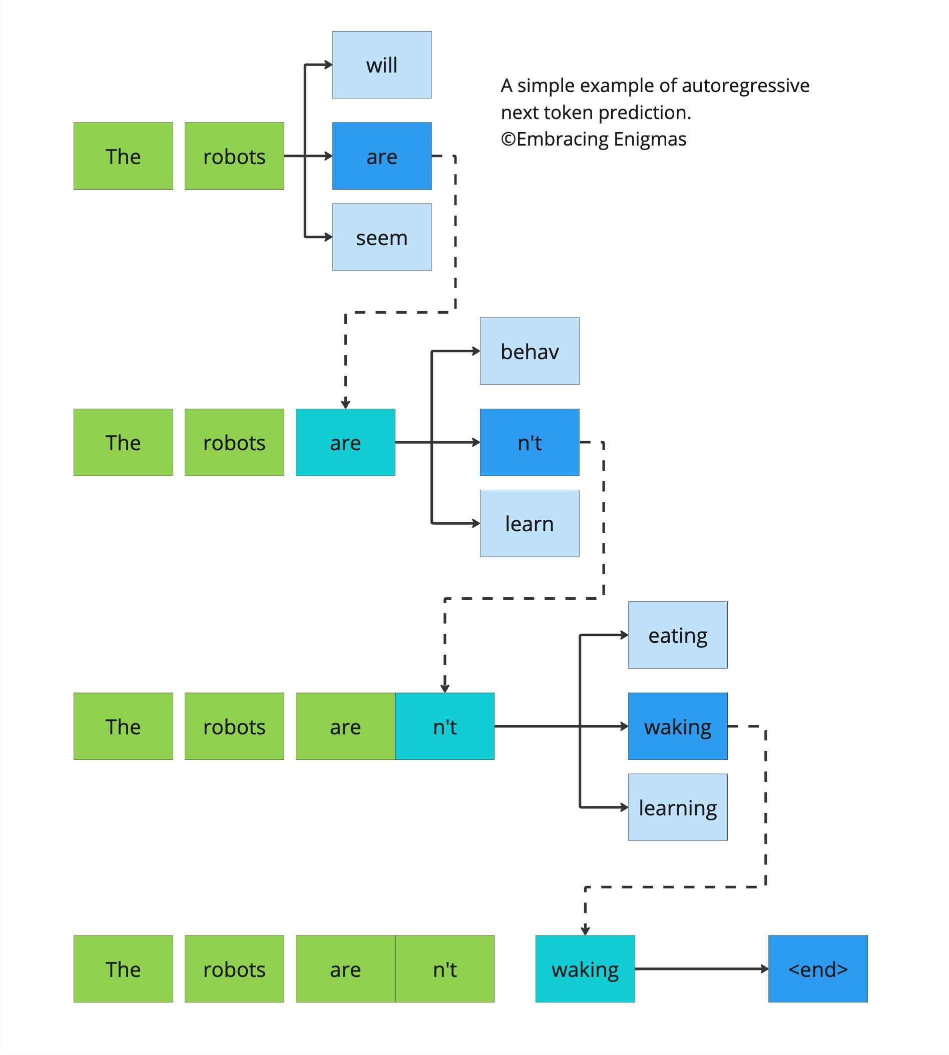
Consider the sentence fragment: "The robots are..."
A language model's task is to calculate a probability distribution over its entire vocabulary to determine the most likely next token. It might assign high probability to tokens like "learning", "behaving", or "sentient", and very low probability to "eating" or "sleeping". Once it selects a token (e.g., "learning"), that token becomes part of the known context for the next step: "The robots are learning..." and the process repeats.
This step-by-step, sequential generation is the essence of autoregressive modeling. The term auto-regressive literally means "regressing on oneself"—the model's own past outputs become its future inputs.
The Probabilistic Foundation: The Chain Rule
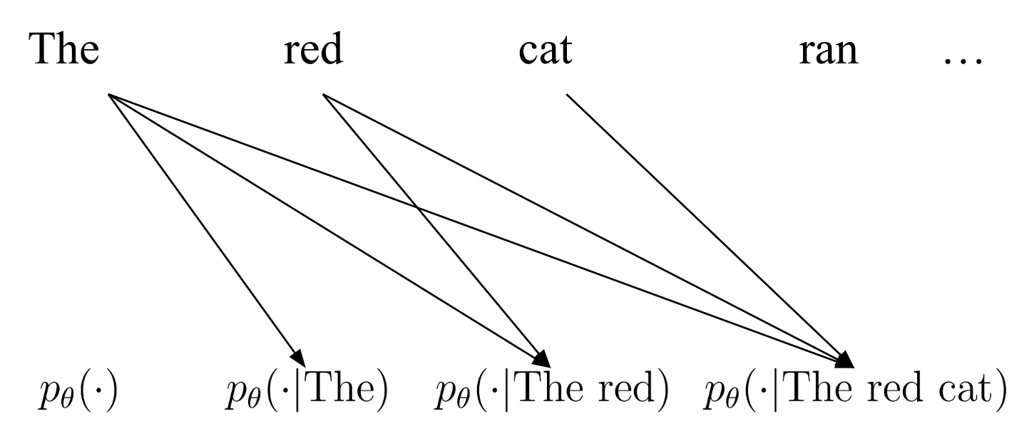
This intuitive process has a rigorous mathematical foundation in probability theory: the chain rule. The chain rule allows us to decompose the joint probability of a sequence of random variables into a product of conditional probabilities.
For a sequence of tokens , the joint probability can be expressed as:
This can be written more compactly as:
Here, is the probability of the -th token given all the tokens that came before it. This formula demonstrates that the complex problem of modeling an entire sequence can be broken down into a series of more manageable next-token prediction problems.
The following video lecture from Stanford provides a clear explanation of how this fundamental rule is the cornerstone of autoregressive models.
Stanford CS236: Deep Generative Models I 2023 I Lecture 3 - Autoregressive Models
This excerpt from a Stanford lecture on Deep Generative Models connects the chain rule of probability to neural autoregressive models.
Watch from the beginning of the section to understand how any joint probability distribution can be factorized using the chain rule, regardless of the ordering of variables. Then, continue from the next segment, which explains how neural networks are used to approximate these conditional probabilities, moving beyond simpler tabular methods to capture complex dependencies.
As the video explains, the power of deep learning comes from using a neural network to model each conditional probability . The network takes the preceding tokens as input and outputs a probability distribution for the next token . The universal approximation theorem gives us confidence that a sufficiently large neural network can learn these complex conditional distributions from data.
The Generation Loop in Practice
The training objective of maximizing the likelihood of sequences in a corpus naturally equips the model for generation at inference time. The process is a direct application of the autoregressive principle.
To see how this works step-by-step, let's turn to a practical demonstration.
This video from HuggingFace clearly explains the architecture of a decoder-only model (like GPT-2) and then walks through the autoregressive generation process.
First, watch the overview of the decoder architecture and its use of masked self-attention from the start. Then, pay close attention to the detailed, step-by-step example of causal language modeling from this section. This part perfectly illustrates the "generation loop" where the model's output is fed back as input.
The process you just saw is the "autoregressive loop":
- Input: Start with a prompt sequence (e.g.,
["My", "name", "is"]). - Process: Pass the sequence through the decoder model.
- Predict: The model outputs a probability distribution over the vocabulary for the token following "is".
- Sample: Select a token from this distribution (e.g., "Clara").
- Append: Add the new token to the end of the sequence (
["My", "name", "is", "Clara"]). - Repeat: Go back to step 2 with the new, longer sequence.
This loop continues until a special end-of-sequence [EOS] token is generated or a predefined length limit is reached.
Connecting the Objective to the Architecture
We've now defined autoregressive language modeling and seen how it works. The final piece of the puzzle is to understand why this objective is intrinsically linked to the decoder-only architecture.
The key is causal masking, a concept we touched upon in Module 2. For the model to learn to predict , it's crucial that during training, the computation for token can only depend on tokens . It must not "peek ahead" at the answer or any subsequent tokens . Causal masking in the self-attention mechanism is the architectural feature that enforces this constraint. It ensures information flows only from left to right, matching the conditional structure of the chain rule.
The following text provides a comprehensive summary, tying together the concepts of decoder architecture, autoregressive generation, and the causal masking that makes it all possible.
Decoder Architecture: Causal Masking & Autoregressive ...
This article offers a clear and detailed explanation of how decoder-only models work, with a focus on the concepts central to this lesson.
Please read the following three sections: First, the section The Decoder-Only Design, which reinforces why this architecture has become standard for generative models. Next, read Understanding Autoregressive Generation. This provides a concise recap of the chain rule and its role in next-token prediction. Finally, read The Causal Masking Requirement. This section is critical as it explains why the architecture must enforce a left-to-right information flow to align with the autoregressive objective.
Conclusion
In this lesson, we have formally defined autoregressive (or causal) language modeling. This is not merely a training task but the fundamental principle that enables modern large language models to generate coherent and contextually relevant text.
Here are the key takeaways:
- Definition: Autoregressive language modeling is the task of sequentially predicting the next token in a sequence, conditioned on all preceding tokens.
- Mathematical Foundation: The task is a direct application of the chain rule of probability, which factorizes the joint probability of a sequence into a product of conditional probabilities.
- Architectural Implementation: This objective is a natural fit for decoder-only Transformer models. The causal mask in the self-attention layer is the crucial component that enforces the required left-to-right information flow, preventing the model from seeing "future" tokens during training.
- Inference: At inference time, the model uses a "generation loop," repeatedly taking its own output as input to generate text token by token.
Having established this foundational training objective, we are now ready to explore the alternative approach. In the next lesson, we will examine masked language modeling, the objective used by encoder-only models like BERT, and see how its bidirectional nature enables a different form of language understanding.