Welcome to our second lesson in the "Decoding Strategies and Inference Optimization" module. In our previous discussion, we demystified the process of autoregressive generation, learning how a model produces text iteratively by feeding its own output back as input. We saw the fundamental loop of predict -> select -> append, but deliberately left the "select" step as a black box.
Today, we will open that box and examine the decision-making process at the heart of text generation. This lesson focuses on two foundational deterministic methods for selecting the next token: greedy search and beam search. Our goal is to compare these strategies, analyzing the trade-offs they make between computational cost and the quality of the generated output. Understanding these deterministic approaches will lay the perfect groundwork for exploring more dynamic, stochastic methods in our next lesson.
Greedy Search: The Path of Least Resistance
The most straightforward strategy for token selection is greedy search. As its name suggests, at each step of the generation process, it simply chooses the single token with the highest probability. It's an entirely deterministic and "short-sighted" approach, always taking the immediately best option without considering future consequences.
Given your background in algorithms, you can think of this as a hill-climbing algorithm on the probability landscape of possible sequences, where each step moves to the highest adjacent point.
The textbook "Dive into Deep Learning" provides a concise formalization of this strategy.
This resource formalizes greedy search and provides a clear example of its sub-optimality.
Please read the section on Greedy Search. Pay close attention to the argmax equation that defines the greedy choice. Then, carefully follow the example illustrated in Figures 10.8.1 and 10.8.2, which demonstrates how choosing a locally sub-optimal token can lead to a globally more probable sequence.
As the reading makes clear, the core issue with greedy search is that the sequence of most likely tokens is not necessarily the most likely sequence overall. The product of probabilities along the greedy path might be lower than an alternative path that involved making a "less optimal" choice early on.
Let's break down the comparison points:
- Computational Cost: Greedy search is highly efficient. At each of the time steps, the model performs one forward pass and finds the
argmaxover the vocabulary . The complexity is therefore , which is linear with respect to the sequence length. This makes it very fast. - Output Quality: While fast, greedy search often produces text that is generic, dull, and prone to repetition. Because it can't "look ahead," it can easily get stuck in loops or commit to a word choice that leads to an awkward or incoherent sentence structure later on. The article from AssemblyAI notes that this method is empirically found to output repetitive text sequences.
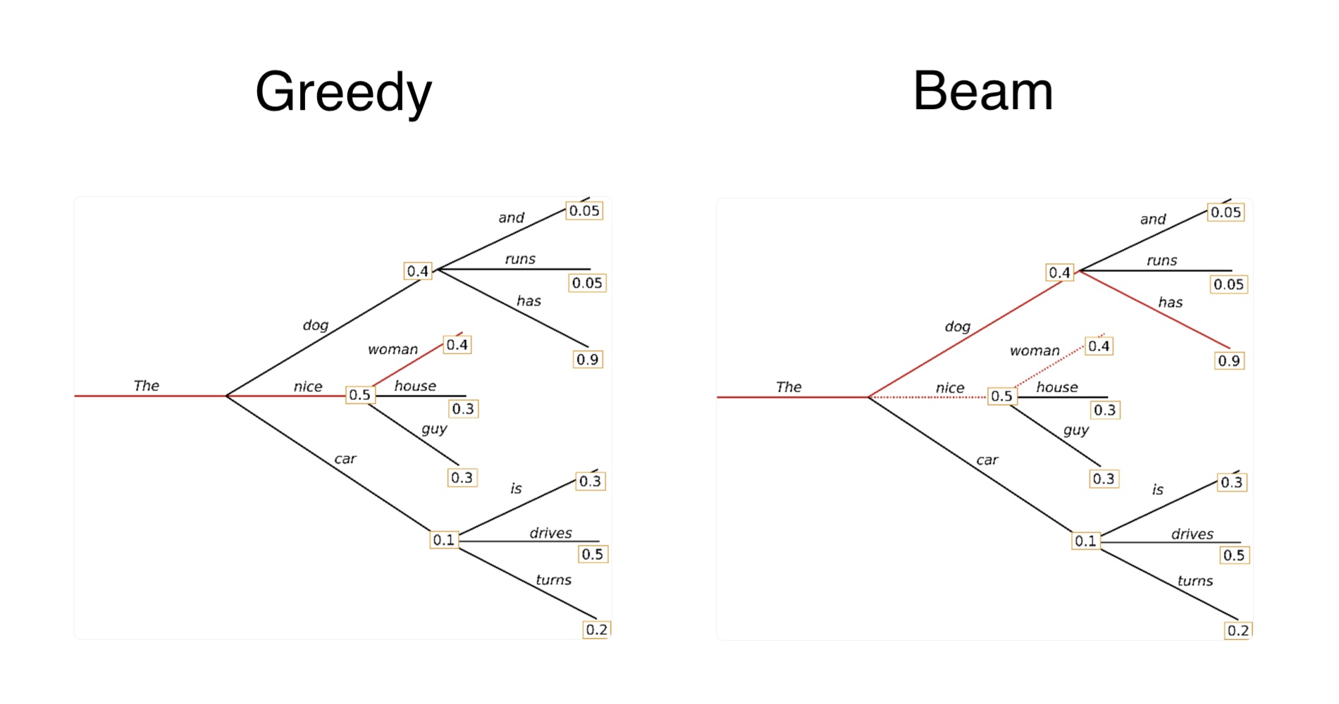
Beam Search: A Wider Path
To mitigate the short-sightedness of greedy search, we can use beam search. This strategy introduces a crucial enhancement: instead of tracking only the single best path, it maintains a "beam" of the most probable partial sequences at each time step. The hyperparameter is known as the beam size or beam width.
This approach is a heuristic search algorithm that explores a much larger portion of the search space than greedy search, without incurring the exponential cost of an exhaustive search (which would explore all possible sequences).
Andrew Ng provides an excellent step-by-step walkthrough of how beam search operates.
This video, "Beam Search" from the Deep Learning Specialization, clearly explains the mechanics of the algorithm.
Please watch the following segments: First, get an overview by watching from the beginning to the introduction. Next, focus on the first step to see how the initial candidates are selected. Finally, and most importantly, watch the detailed explanation of the second and subsequent steps. Pay close attention to how the algorithm generates k * |V| candidates and then prunes them back down to the top k to form the new beam.
The process described in the video can be summarized as follows:
- Step 1: Generate probabilities for the first token. Select the top tokens and place these one-token sequences into the beam.
- Step 2: For each of the sequences currently in the beam, generate the probability distribution for the next token. This gives you potential two-token sequences.
- Step 3: Calculate the total probability for each of these candidate sequences. The probability of a sequence is .
- Step 4: From this large set of candidates, select the sequences with the highest total probabilities. These become the new beam.
- Repeat: Continue this process until an end-of-sequence token is generated for all sequences in the beam or a maximum length is reached.
The following diagram provides a clear, static illustration of this process with a beam size of .

A Formal Comparison
Now we can directly compare the two strategies based on our learning objective.
| Aspect | Greedy Search | Beam Search |
|---|---|---|
| Algorithm | At each step, select the single most probable next token. | At each step, maintain k most probable sequences and expand them. |
| Computational Cost | $\mathcal{O}( | \mathcal{Y} |
| Output Quality | Often low. Prone to repetition and logical errors due to its myopic nature. | Generally higher than greedy. Finds more probable, coherent sequences by "looking ahead". |
| Determinism | Fully deterministic. | Fully deterministic for a given k. |
| Relationship | A special case of beam search where the beam size k=1. |
A generalization of greedy search. |
The crucial insight is the trade-off. Beam search offers a significant quality improvement over greedy search at a linearly increasing computational cost determined by the beam size k.
To finalize the comparison, let's revisit Andrew Ng's conclusion.
Watch this short clip from the conclusion, where he explicitly states that greedy search is beam search with a beam width of one.
Limitations and The Scoring Function
While beam search is an improvement, it's not a panacea. For open-ended creative text generation, it can still produce text that feels safe, repetitive, and lacks the natural variance of human writing. This is because it is still fundamentally optimized to find high-probability sequences.
A final important detail is how sequences are scored. Multiplying many small probabilities can lead to numerical underflow. Therefore, in practice, we use log-probabilities. The goal becomes to find the sequence that maximizes the sum of log-probabilities.
However, this sum naturally favors shorter sequences. To counteract this, a length penalty is often introduced. The final score to maximize is:
Here, is the sequence length and is a hyperparameter (often around 0.75) that controls the strength of the penalty on longer sequences.
Conclusion
In this lesson, we have moved from the "what" of autoregressive generation to the "how" of token selection. We've contrasted two fundamental deterministic decoding strategies.
Here are the key takeaways:
- Greedy Search: The simplest, fastest method. It picks the most likely token at each step, but its short-sightedness often leads to suboptimal and repetitive final sequences.
- Beam Search: A more robust heuristic that improves output quality by maintaining a "beam" of candidate sequences. It offers a direct trade-off between computational cost (linear in
k) and search quality. - Greedy as a Special Case: You can view greedy search as simply beam search with a beam size of
k=1. - Deterministic Limitations: Both methods are deterministic and tend to favor high-probability, "safe" text, which may lack the diversity and creativity expected in many applications.
We have now established a solid understanding of how to find the most likely sequences. But what if we don't always want the most likely? What if we want to introduce creativity, surprise, or controlled randomness? This question leads us directly to our next topic: stochastic decoding strategies, where we will explore methods like temperature scaling, top-k sampling, and nucleus sampling.