Understanding GELU in Feed-Forward Networks

Introduction

In our last lesson, we established the position-wise feed-forward network (FFN) as the Transformer's computational engine, providing both essential non-linearity and a storage mechanism for learned knowledge. We used the familiar Rectified Linear Unit (ReLU) as a placeholder for the activation function. While simple and effective in many contexts, ReLU has limitations that can hinder the performance of large, sophisticated models.

This lesson delves into the Gaussian Error Linear Unit (GELU), the activation function that replaced ReLU in seminal Transformer models like BERT and GPT-2, becoming a new standard. We will explore why this change was necessary by first examining the shortcomings of ReLU. Then, we will uncover the elegant mathematical and intuitive foundation of GELU, understanding it as a smooth, probabilistic version of ReLU. By the end, you will be able to explain GELU's key properties—such as its smoothness and non-monotonicity—and articulate why it contributes to the stability and superior performance of modern LLMs.

From a Hard Gate to a Smooth Weighting: The Limitations of ReLU

You'll recall from your deep learning background that the ReLU function, defined as $ReLU (x) = max (0, x)$ , acts as a simple gate: it passes positive values through and shuts off negative values completely. This simplicity is powerful but comes with drawbacks, particularly in deep and complex networks.

The most cited issue is the "dying ReLU" problem. When a neuron's input is negative, its output is zero. Crucially, the gradient of the ReLU function for negative inputs is also zero. This means that if a neuron consistently receives negative inputs, its weights will no longer receive gradient updates during backpropagation. The neuron effectively "dies" and ceases to participate in learning.

To see a clear explanation of this and other issues, let's watch a short video segment.

GELU Activation Function in the LLM Architecture

This video provides a concise review of the ReLU function and clearly explains its primary disadvantages, which directly motivate the need for a more advanced activation like GELU.

Please watch from this point. Focus on the two main problems identified: the sharp, non-differentiable point at zero and the "dead neuron" problem caused by zero gradients for all negative inputs.

The abrupt switch at $x = 0$ and the complete nullification of negative inputs represent a "hard", deterministic gating mechanism. An ideal function might offer a "softer," more nuanced transition and allow for richer gradient signals, especially around zero. This is precisely what GELU provides.

The GELU Formulation: Probabilistic Gating

The insight behind GELU, introduced by Hendrycks and Gimpel in 2016, is to replace ReLU's deterministic gating (multiply by 0 or 1 based on sign) with a form of probabilistic gating. Instead of gating based only on the input's sign, GELU weights an input by its value, specifically, by how large it is compared to other inputs under a standard normal distribution.

The core idea is to model the activation as a stochastic process. We can multiply a neuron's input, $x$ , by a random binary mask, $m$ , where $m$ is drawn from a Bernoulli distribution. The probability of the mask being 1 (i.e., preserving the input) depends on the input itself.

Specifically, $m \sim Bernoulli (Φ (x))$ , where $Φ (x)$ is the cumulative distribution function (CDF) of the standard normal distribution, $N (0, 1)$ . The CDF $Φ (x)$ gives the probability that a random variable from $N (0, 1)$ is less than or equal to $x$ .

Since we want a deterministic function for our network, we take the expectation of this stochastic process. The GELU activation is defined as the expected value of the input $x$ after being masked:

GELU (x) = E [x \cdot m] = x \cdot P (m = 1) + 0 \cdot P (m = 0) = x Φ (x)

This is a profound idea: GELU scales an input $x$ by the probability that it is greater than a random input from a standard normal distribution.

To dig into this foundational concept, we will go directly to the source.

[PDF] Gaussian Error Linear Units (GELUs) - arXiv

This is the original paper that proposed GELU. Reading the formulation section will give you a first-hand account of the motivation and derivation, connecting it to concepts like dropout and zoneout.

Please read the section titled GELU Formulation. Your focus should be on understanding how the authors combine the properties of ReLU and dropout to arrive at the stochastic formulation with the Bernoulli mask, and how taking the expectation of this process yields the final deterministic function, x\Phi(x).

From Theory to Practice: The Math of GELU

The definition $x Φ (x)$ is elegant, but how do we compute it? The Gaussian CDF, $Φ (x)$ , does not have a simple closed-form expression. However, it can be expressed using the Gauss error function, denoted $erf (x)$ .

The relationship is:

Φ (x) = \frac{1}{2} (1 + erf (\frac{x}{2}))

Substituting this into our definition gives the exact mathematical formula for GELU:

GELU (x) = x \cdot \frac{1}{2} (1 + erf (\frac{x}{2}))

While exact, the error function is computationally intensive. In practice, especially in performance-critical LLMs, fast approximations are used. The approximation used in GPT-2 and many subsequent models is based on the hyperbolic tangent function ( $tanh$ ):

GELU (x) \approx 0.5 x (1 + tanh [2/ π (x + 0.044715 x^{3})])

This formula may look complex, but it's composed of standard mathematical operations that are highly optimized on modern hardware (like GPUs), making it much faster to compute than the exact erf-based version.

The following video walks through both the mathematical definition and the practical approximation.

GELU Activation Function in the LLM Architecture

This video bridges the gap between the theoretical concept of GELU and its practical implementation, explaining both the exact formula and the widely used approximation.

First, watch the segment on the mathematical representation, which introduces the x\Phi(x) formula. Then, watch the next segment on the GPT-2 approximation, which presents the tanh-based formula.

Key Properties and Advantages of GELU

Now that we understand what GELU is and how it's calculated, let's analyze its properties, which explain its effectiveness.

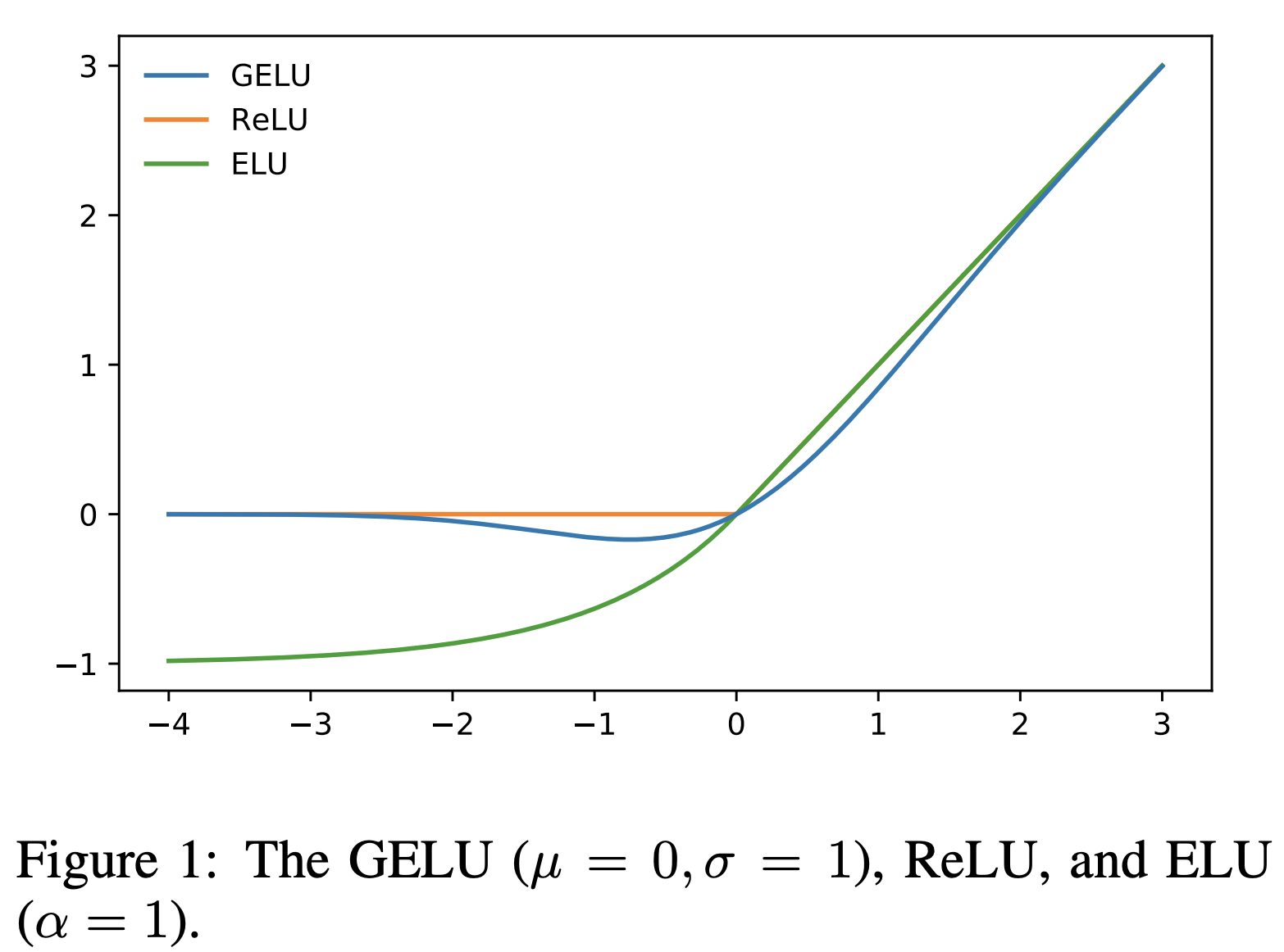
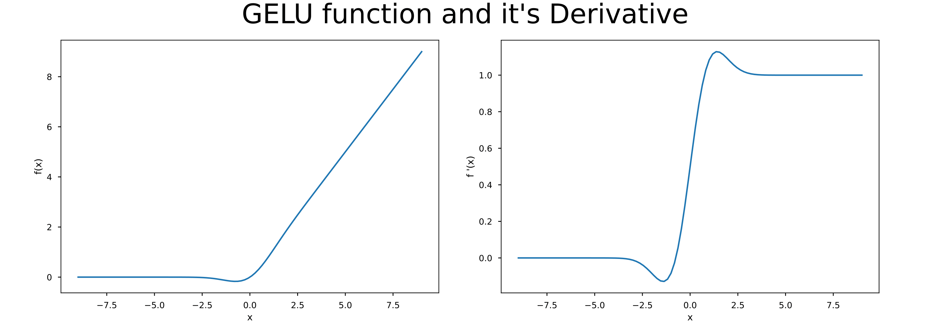
A comparison of GELU (blue), ReLU (orange), and another common activation, ELU (green). Notice how GELU smoothly approximates ReLU for large positive values but behaves very differently for negative values and values near zero.

Smoothness and Differentiability: Unlike ReLU's sharp corner, GELU is a smooth function, differentiable everywhere. This provides a clean, non-zero gradient for almost all input values, which is beneficial for gradient-based optimization algorithms like Adam. It avoids the abrupt changes in gradient that can make training unstable.

The GELU function (left) and its derivative (right). The derivative is smooth and bell-shaped, peaking near x=0, providing a rich gradient signal in this critical region, unlike ReLU's zero gradient for x<0.

Non-Monotonicity (The "Negative Dip"): A unique feature of GELU is that it is non-monotonic. As you can see in the plots, it dips slightly into negative territory for small negative inputs before rising back toward zero. This means that for some negative inputs, it can actually "flip" the sign. This behavior, which is absent in ReLU and ELU, can be seen as a form of implicit regularization. It provides a more complex and expressive mapping, allowing the network to potentially capture more intricate patterns than a simple monotonic function.
Probabilistic Interpretation: At its core, GELU "weights its input depending upon how much greater it is than other inputs" (Hendrycks & Gimpel, 2016). For large positive $x$ , $Φ (x) \approx 1$ , so $GELU (x) \approx x$ , behaving like an identity function. For large negative $x$ , $Φ (x) \approx 0$ , so $GELU (x) \approx 0$ , behaving like ReLU's zeroing-out. The smooth transition between these regimes is what makes it so powerful.
Empirical Performance: Most importantly, GELU simply works better in practice for Transformers. As noted in the original paper's appendix, "Things changed as the GELU began to be used in BERT and GPT, becoming the default activation for state-of-the-art Transformers." This superior empirical performance is the ultimate reason for its widespread adoption.

The article below provides a fantastic summary and quantitative comparison of these properties.

FFN Activation Functions: ReLU, GELU, and SiLU for Transformer ...

This article offers an excellent, detailed analysis of GELU, including its intuition, mathematical properties, and the significance of its unique shape.

First, read the introduction to GELU in the section The Smooth Alternative. Then, jump to the section The Negative Dip for an insightful discussion on non-monotonicity as implicit regularization. Finally, read the Summary for GELU at the end of the article for a concise wrap-up.

Conclusion

In this lesson, we have replaced the simple ReLU activation with the more sophisticated and powerful GELU. You now understand that this is not just an arbitrary choice, but a principled one rooted in addressing the limitations of older activation functions.

Here are the key takeaways:

Motivation: GELU was developed to overcome the "dying ReLU" problem and provide a smoother, more robust activation function suitable for deep networks.
Core Concept: GELU is defined as $x Φ (x)$ , which can be interpreted as weighting an input by its probability of being positive under a standard normal distribution. It is a deterministic function that approximates a stochastic regularization effect.
Key Properties: GELU is smooth, differentiable everywhere, and non-monotonic (featuring a characteristic "negative dip"). This combination allows for richer gradient flow and potentially more complex function approximation.
Practical Use: Due to its superior empirical performance, GELU (or its fast tanh approximation) became the standard activation function in the FFN layers of foundational Transformer models like BERT and GPT-2.

We have now examined the two main sub-layers of the Transformer block—multi-head attention and the position-wise feed-forward network (now refined with GELU). However, simply stacking these layers would lead to an unstable and untrainable network. In our next lesson, we will explore residual connections, a simple yet crucial technique that enables information to flow through deep networks and mitigates the infamous vanishing gradient problem.