Multi-Head Attention: Computation, Concatenation, and Projection

The Multi-Head Attention Pipeline

At its core, multi-head attention consists of four main steps, which we will explore in detail:

1. Initial Linear Projections: Create distinct Query, Key, and Value sets for each head.
2. Parallel Attention Computation: Apply scaled dot-product attention independently to each head.
3. Concatenation: Combine the outputs of all heads.
4. Final Linear Projection: Mix the combined outputs to produce the final result.

The entire process is visualized in the diagram below. We start with the input token embeddings (represented as Q, K, and V for simplicity, as they are all derived from the same source in self-attention) and end with the final Multi-Head Attention Output.

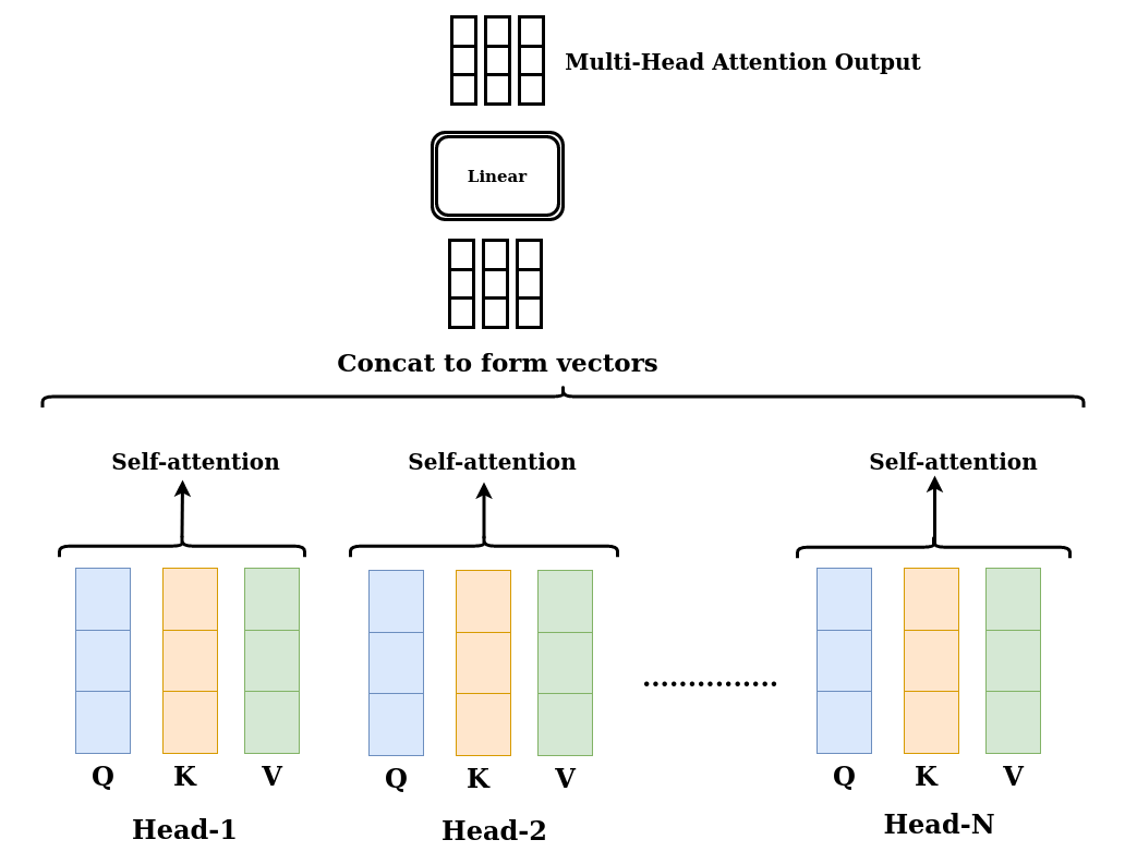
Let's break down each stage.

1. Initial Linear Projections

In the last lesson, we mentioned that each head operates in a separate "representation subspace." This is achieved through linear projections.

Let's say our input is a matrix $X$ of token embeddings, with dimensions $[\text{sequence length},d_{\text{model}}]$, where $d_{\text{model}}$ is the embedding dimension (e.g., 512). If we have $h$ attention heads, we don't just use one set of weight matrices $W^Q,W^K,W^V$. Instead, we create $h$ independent sets of them:

• $W_i^Q$, $W_i^K$, $W_i^V$ for each head $i\in \{1,\dots ,h\}$.

A crucial architectural detail is that the output dimension of these projections is smaller than $d_{\text{model}}$. Typically, the dimension for each head's keys, queries, and values is set to $d_k=d_v=d_{\text{model}}/h$. For example, with a model dimension of 512 and 8 heads, each head would work with vectors of dimension 64.

For each head $i$, we compute its query, key, and value matrices:
$Q_i=X{W}_i^Q(W_i^Q\in {\mathbb{R}}^{d_{\text{model}}\times d_k})$
$K_i=X{W}_i^K(W_i^K\in {\mathbb{R}}^{d_{\text{model}}\times d_k})$
$V_i=X{W}_i^V(W_i^V\in {\mathbb{R}}^{d_{\text{model}}\times d_v})$

Because each $W_i$ matrix is initialized randomly and updated independently during training, each head learns a unique projection, effectively focusing on a different subspace of the original embedding. This is the foundation of the specialization we discussed previously.

2. Parallel Attention Computation

With the projected $Q_i,K_i,V_i$ for each head, we can now perform scaled dot-product attention in parallel. The calculation for each head is exactly what you learned in the previous module:

${\text{head}}_i=\text{Attention}(Q_i,K_i,V_i)=\text{softmax}\left(\frac{Q_i{K}_i^T}{\sqrt{d_k}}\right)V_i$

Since these $h$ computations are independent of one another, they are perfectly suited for parallelization on modern hardware like GPUs. The output of each head, ${\text{head}}_i$, is a matrix of size $[\text{sequence length},d_v]$.

3. Concatenation

After each of the $h$ heads has produced its output matrix, we need to combine them back into a single matrix. This is done by simple concatenation along the feature dimension:

$\text{Concat}({\text{head}}_1,{\text{head}}_2,\dots ,{\text{head}}_h)$

The resulting matrix has dimensions $[\text{sequence length},h\times d_v]$. Since we chose $d_v=d_{\text{model}}/h$, the dimension of this concatenated matrix becomes $[\text{sequence length},d_{\text{model}}]$. We have successfully returned to the original embedding dimension of our model, but now the representation for each token is a composite of information from all the specialized heads.

4. Final Linear Projection

The concatenated output contains rich information, but the outputs from each head are still segregated in their own "lanes." To allow these specialized representations to be integrated and mixed, we apply one final linear projection using another learned weight matrix, $W^O\in {\mathbb{R}}^{d_{\text{model}}\times d_{\text{model}}}$:

$\text{MultiHead}(Q,K,V)=\text{Concat}({\text{head}}_1,\dots ,{\text{head}}_h)W^O$

This final layer allows the model to learn how to best combine the outputs of the different heads. It can choose to weigh some heads' outputs more heavily than others, creating a powerful, unified representation. The output of this operation is the final output of the multi-head attention sub-layer, and it has the dimensions $[\text{sequence length},d_{\text{model}}]$, ready to be passed to the next layer in the Transformer block.

A Guided Walkthrough of the Mechanism

To solidify your understanding, we will now walk through this process using a combination of video explanations, formal definitions, and code implementations.

First, let's watch a clear, step-by-step visual explanation of the entire pipeline we just discussed.

Next, let's ground this visual intuition in a more formal mathematical description and a concrete PyTorch implementation. The following tutorial provides a concise and comprehensive look at the subject.

The approach of using a single large qkv_proj matrix and then reshaping is a common and efficient implementation trick. It's computationally equivalent to having separate $W_i^Q,W_i^K,W_i^V$ matrices for each head but can be faster in practice.

Finally, to see this from a "from-scratch" perspective that deeply aligns with your goals, let's watch how Andrej Karpathy implements multi-head attention.

Conclusion

In this lesson, we have demystified the inner workings of multi-head attention. We moved from the high-level motivation of "why" to the detailed mechanics of "how." By breaking down the process, we can see it's a sequence of logical, well-motivated steps rather than a single monolithic black box.

Here are the key takeaways on the mechanics of multi-head attention:

• Projection into Subspaces: The process begins by projecting the input embeddings into lower-dimensional query, key, and value representations for each of the $h$ heads using independent weight matrices ($W_i^Q,W_i^K,W_i^V$).
• Parallel Computation: Scaled dot-product attention is performed independently and in parallel for each head, allowing for specialization.
• Concatenation and Projection: The outputs of all heads are concatenated back into a single, full-dimension tensor. A final linear projection ($W^O$) is then applied to integrate the information from all the specialized heads into a unified output.
• Dimensionality: The dimensions are carefully managed throughout. By setting $d_{\text{head}}=d_{\text{model}}/h$, the total computational cost of multi-head attention is roughly equivalent to that of a single attention head operating on the full $d_{\text{model}}$ dimension.

You have now mastered the first major component of a Transformer block. However, the multi-head attention sub-layer does not work in isolation. In the next lesson, we will explore the second key component: the Position-wise Feed-Forward Network, and see how it works in tandem with attention to process the information for each token.