Multi-Criteria Calculations with SUMIFS and COUNTIFS

From One Condition to Many: Introducing SUMIFS and COUNTIFS

You already have some experience with SUMIF, which lets you sum values based on a single rule. But real-world analysis almost always requires you to filter by several conditions at once. This is where SUMIFS and COUNTIFS become essential.

• SUMIFS sums values in a range that meet multiple 'AND' conditions.
• COUNTIFS counts the number of cells that meet multiple 'AND' conditions.

While their names are similar to their single-condition counterparts, there's a key difference in their structure that's important to grasp. The following video provides an excellent introduction. The presenter, Leila Gharani, makes a strong case for why you should almost always prefer the IFS versions, even for a single condition.

The most critical takeaway is the change in syntax, especially for SUMIFS. Unlike SUMIF, where the range to be summed is the last argument, in SUMIFS it's the very first.

SUMIFS(sum_range, criteria_range1, criteria1, criteria_range2, criteria2, ...)

This structure allows the function to accept a variable number of criteria pairs. Let's see it in action.

Performing Multi-Criteria Sums with SUMIFS

Imagine you have a sales table and need to find the total sales for a specific product in a given month. This requires two conditions.

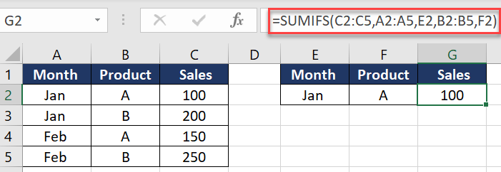
Let's break down the formula shown in the image above: =SUMIFS(C2:C5, A2:A5, E2, B2:B5, F2)

1. C2:C5 (sum_range): This is the range containing the numbers we want to add up—the 'Sales' column.
2. A2:A5 (criteria_range1): This is the first range to check our condition against—the 'Month' column.
3. E2 (criteria1): This is the first condition. The formula checks which cells in A2:A5 are equal to the value in cell E2 ("Jan").
4. B2:B5 (criteria_range2): This is the second range to check—the 'Product' column.
5. F2 (criteria2): This is the second condition. The formula checks which cells in B2:B5 are equal to the value in cell F2 ("A").

The function only sums the value from column C if both conditions for that row are met.

The video you just saw explains this process clearly. Let's revisit it to see a guided walkthrough of building a SUMIFS formula with two and then three criteria.

Counting with Multiple Criteria using COUNTIFS

COUNTIFS follows the same logic but is simpler because you're just counting rows, not summing a separate column. Therefore, it doesn't need a sum_range.

COUNTIFS(criteria_range1, criteria1, criteria_range2, criteria2, ...)

This function is perfect for answering questions like, "How many orders were delivered within a specific date range?" The image below shows a practical example of this.

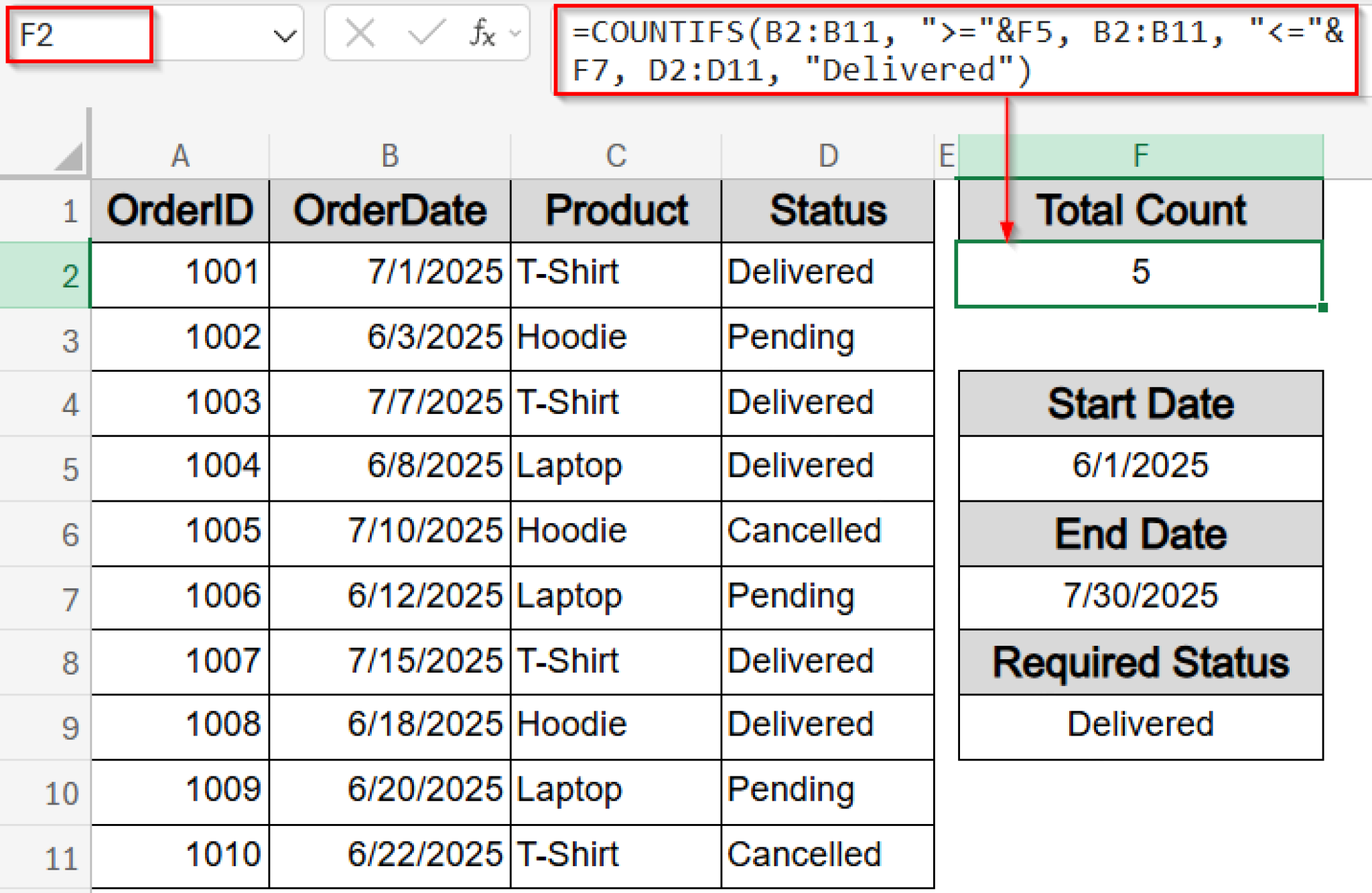
Let's analyze the formula: =COUNTIFS(B2:B11, ">="&F5, B2:B11, "<="&F7, D2:D11, "Delivered")

1. B2:B11, ">="&F5: The first condition pair checks if the OrderDate is greater than or equal to the Start Date in cell F5.
2. B2:B11, "<="&F7: The second pair checks if the same OrderDate is less than or equal to the End Date in cell F7.
3. D2:D11, "Delivered": The third pair checks if the Status is "Delivered".

A row is only counted if it satisfies all three of these conditions. Notice the syntax for the date criteria (">="&F5). We'll explore these operators next.

Mastering Criteria: Operators and Wildcards

To unlock the full potential of SUMIFS and COUNTIFS, you need to be comfortable with advanced criteria syntax.

Comparison Operators

You can use operators like > (greater than), < (less than), and <> (not equal to). The key is to remember that the operator and the value must be enclosed in quotation marks, like ">500".

If you're comparing against a value in another cell (which is a best practice), you must concatenate the operator and the cell reference using an ampersand (&), like ">"&G1.

Wildcards

Wildcards allow for partial text matching, which is incredibly useful when your data isn't perfectly uniform. This directly leverages the data cleaning skills from our last lesson!

• * (asterisk) matches any number of characters. For example, "Shirt*" would match "Shirt White", "Shirt Blue", and "Shirt".
• ? (question mark) matches exactly one character.

This next video segment provides a fantastic, clear walkthrough of using both comparison operators and wildcards in your formulas.

For a quick reference, the article below contains a very helpful summary table of the different criteria types you can use. It's a great page to bookmark.

Best Practices and Troubleshooting

As you use these functions more, you'll inevitably run into errors or unexpected results. The most common issues are mismatched range sizes (which cause a #VALUE! error) and incorrect criteria formatting.

The following reading from DataCamp covers these common pitfalls and provides excellent best practices, such as using cell references instead of hardcoding criteria. Adopting these habits early will make your spreadsheets more robust and easier to manage.

Conclusion

In this lesson, you've added two of Excel's most powerful analytical functions to your toolkit. You've moved from single-condition aggregation to sophisticated multi-criteria analysis, a skill that is fundamental to data analysis.

Here are the key takeaways:

• SUMIFS and COUNTIFS allow you to aggregate or count data based on multiple 'AND' conditions.
• The syntax is key: SUMIFS requires the sum_range as its first argument, while COUNTIFS has no sum_range.
• Mastering criteria is crucial. This includes using comparison operators (">500", ">"&A1), wildcards ("Shirt*"), and correctly formatting date ranges.
• Following best practices, like using cell references for criteria and ensuring all ranges are the same size, makes your analysis more flexible and less error-prone.

In our next lesson, we will shift from aggregation to retrieval. You'll learn how to use INDEX-MATCH to perform flexible, powerful lookups that can pull a specific piece of information from a dataset based on one or more criteria. This will complement your new SUMIFS skills and further expand your data manipulation capabilities.