Welcome to the next lesson in our Advanced Excel module. In the previous session, you learned how to use IF and IFS functions to create new categories in your data based on logical rules. This is a crucial data preparation step, and today you'll see how to use those categories—and others already in your dataset—to perform powerful analysis.
This lesson introduces one of the most essential tools for any data analyst: the PivotTable. If you've ever used a GROUP BY statement in SQL or dragged dimensions and measures into a view in Tableau or Power BI, you will find the concept of a pivot table very familiar. It is Excel's primary tool for interactively summarizing, aggregating, and exploring large datasets without writing a single formula.
Our goal for this lesson is to learn how to create a pivot table to summarize data by one or more categorical variables and customize its calculations. By the end of this 60-minute session, you will be able to transform a raw table of data into a dynamic summary report, a core skill for answering business questions efficiently.
What is a PivotTable?
At its heart, a pivot table takes your flat, tabular data and "pivots" it to create a structured summary. Imagine you have a large list of sales transactions, with columns for Region, Product, and Sales Amount. A pivot table can instantly answer questions like:
- What are the total sales for each region?
- Which products are the top sellers in each region?
- How many transactions were there for each product category?
This process of aggregation and grouping is fundamental to data analysis. Given your experience with SQL, you can think of a pivot table as a visual and interactive way to execute a GROUP BY query.
The video below from Alex The Analyst provides an excellent introduction. He makes a direct comparison to tools like Tableau, which should align well with your experience. Pay close attention to his overview of the dataset and the initial setup.
Pivot Tables in Excel | Excel Tutorials for Beginners
Watch the beginning of this video to understand the purpose of pivot tables and see how one is inserted into a new worksheet.
Watch from the introduction at the beginning to see why pivot tables are so pivotal for analysts. Then, follow his walkthrough from inserting a pivot table to the point where the blank pivot table and the "PivotTable Fields" pane appear.
The Anatomy of a PivotTable
As you saw in the video, once you create a pivot table, you work with the PivotTable Fields pane. This pane is your control center and is organized into four key areas. Your experience with data visualization tools will make this interface feel intuitive:
- Rows: Drag categorical fields here to create row labels in your summary table (e.g., a list of countries). This is analogous to the dimensions you would place on the Rows shelf in Tableau.
- Columns: Drag categorical fields here to create column headers (e.g., a series of years).
- Values: This area is for the numeric fields you want to aggregate. It performs the calculation, like
SUM(Sales)orCOUNT(Orders). This is the equivalent of the measures or metrics you analyze. - Filters: Fields placed here allow you to filter the entire pivot table report by one or more criteria (e.g., filter the entire sales report to show only "Female" customers).

Creating a Summary with One or More Categories
Let's build a pivot table step-by-step. The most critical first step is ensuring your data is well-structured.
Create a PivotTable to analyze worksheet data
Before creating any pivot table, it's essential to prepare your data correctly. This official Microsoft guide outlines the best practices.
Please read the section titled Data format tips. The most important takeaway is to format your data as an Excel Table (Insert > Table or Ctrl+T) before creating the pivot table. This makes your pivot table dynamic, so it automatically includes new data you add later.
Once your data is in an Excel Table, you can insert a pivot table. Now, let's build a summary. We'll start by looking at revenue by country and then drill down further.
The following video segment clearly demonstrates adding a categorical field to the Rows area, a numeric field to the Values area, and then adding a second categorical field to create a hierarchical, drill-down summary.
Pivot Tables in Excel | Excel Tutorials for Beginners
This part of the video shows you how to populate the pivot table to create a meaningful summary, starting with a simple one-level grouping and then adding a second level.
First, watch how to create a hierarchical view by adding Country and State to the Rows area, from . Notice the expand/collapse functionality, which is similar to drill-downs in BI tools. Next, see how adding Revenue to the Values area completes the summary, from . He also covers basic number formatting here.
This multi-level structure in the 'Rows' area is extremely powerful. For example, you could analyze Product_Category, then Sub_Category, then Product_Name to see performance at different levels of granularity.
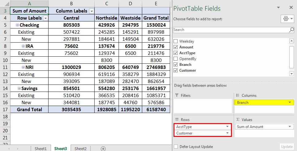
You can also create a two-dimensional summary by using the Columns area. For instance, if you drag 'Country' to Rows and 'Year' to Columns, you'll get a matrix showing the revenue for each country across different years.
Customizing Summary Calculations
By default, Excel will SUM numeric fields and COUNT text-based fields you place in the Values area. However, as a data analyst, you'll often need other aggregations like averages, counts of unique items, or maximum values.
You can change this calculation through the Value Field Settings. The process is straightforward:
- Click the dropdown arrow on the field in the Values area.
- Select "Value Field Settings...".
- In the dialog box, choose the calculation you need from the "Summarize value by" list (e.g., Count, Average, Max, Min).
- You can also change the display name of the field in this dialog box to make your report clearer (e.g., change "Sum of Revenue" to "Total Revenue").
This article from DataCamp provides a clear, hands-on example of creating a simple pivot table and then changing the default aggregation from SUM to COUNT.
Working with PivotTables in Excel
This blog post provides a practical example of building a pivot table and adjusting its settings.
Read the sections titled Adding your data. Focus on how the author drags Country to Rows and Customer_Age to Values, and then crucially, how they change the summary calculation from Sum to Count.
The next video segment also provides a fantastic walkthrough of these options, including not only changing the calculation but also showing values as a percentage of the total—a very common analytical task.
Pivot Tables in Excel | Excel Tutorials for Beginners
Watch this segment to see how to access the 'Value Field Settings' and change how your data is summarized and displayed.
From , watch how Alex changes the summary calculation and also shows the value as a percentage of the grand total. This demonstrates the flexibility of the Values area.
Conclusion
In this lesson, we've moved from simple formulas to one of Excel's most powerful analytical features. Pivot tables are the foundation of exploratory data analysis in a spreadsheet environment, allowing you to quickly reshape and summarize your data to uncover insights.
Here are the key takeaways:
- Pivot tables are interactive tools for summarizing large datasets, analogous to SQL's
GROUP BYor the functionality of BI tools like Tableau. - The PivotTable Fields pane, with its Rows, Columns, Values, and Filters areas, is where you build your report.
- Always start with clean, tabular data, and use Excel's Table feature (
Ctrl+T) to ensure your pivot table can be easily refreshed with new data. - You can create complex summaries by dragging multiple categorical variables into the Rows or Columns areas to create hierarchies and cross-tabulations.
- The Value Field Settings allow you to customize your summary by changing the calculation from the default
SUMorCOUNTtoAVERAGE,MAX,MIN, and more.
You now have the ability to create a summary report from raw data. In our next lesson, we will build on this foundation by learning how to filter, sort, and group data within a pivot table. This will enable you to refine your reports and zero in on the specific information needed to answer precise business questions.