Qubit Representation on the Bloch Sphere

From Two Complex Numbers to Two Angles

As we recap from the last lesson, a general qubit state $|\psi ⟩=\alpha |0⟩+\beta |1⟩$ is defined by two complex numbers, $\alpha$ and $\beta$. Since a complex number has a real and an imaginary part, this seems to imply we need four real numbers to fully describe the state. However, the Bloch sphere is a standard 3D sphere that can be described with just two angles, like latitude and longitude on Earth. How can we reconcile these two descriptions?

The answer lies in two constraints on the quantum state that we've encountered before:

1. The Normalization Constraint: The state vector must have a unit length, meaning $|\alpha {|}^2+|\beta {|}^2=1$. This is one mathematical constraint that reduces the number of free parameters from four to three.
2. The Global Phase Constraint: A quantum state is physically equivalent if it is multiplied by a global phase factor, $e^{i\gamma }$. For example, the state $e^{i\gamma }|\psi ⟩$ is physically indistinguishable from $|\psi ⟩$. This means we can always factor out one of the phases, effectively removing another degree of freedom.

With these two constraints, we are left with only two real, independent parameters needed to define any single-qubit state. These two parameters can be beautifully mapped to the two angles of a spherical coordinate system.

The following video provides an excellent walkthrough of this dimensional reduction, showing how we start with four apparent degrees of freedom and logically arrive at the two that define a point on the Bloch sphere.

The Bloch Sphere Representation

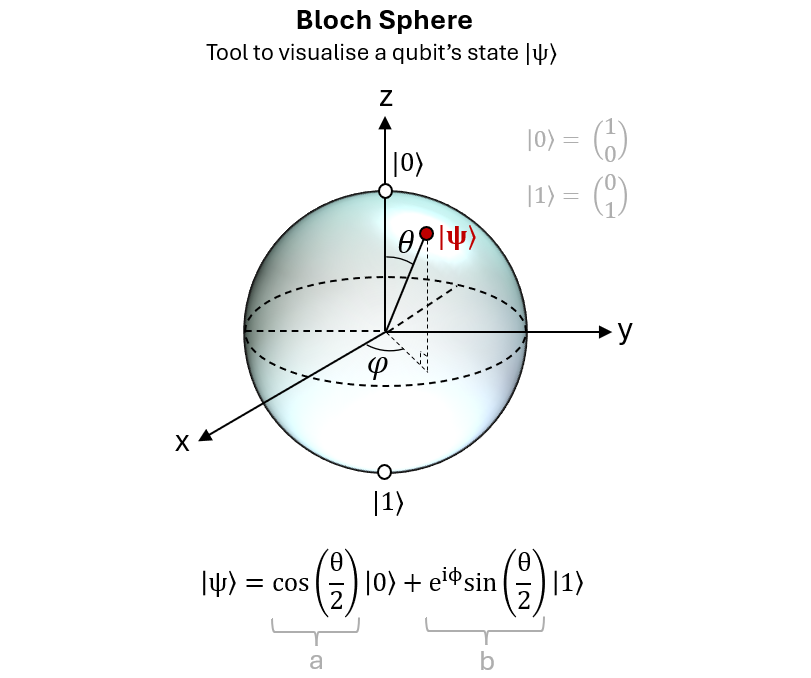
The video demonstrated how the state of a qubit can be parameterized by two angles, $\theta$ and $\varphi$. This gives rise to the standard Bloch sphere representation of a qubit state:

Here:

• $\theta$ is the polar angle, measured from the positive z-axis. It ranges from $0\le \theta \le \pi$.
• $\varphi$ is the azimuthal angle, measured from the positive x-axis in the xy-plane. It ranges from $0\le \varphi <2\pi$.

This equation maps every pure state of a single qubit to a unique point on the surface of a unit sphere.

For a more rigorous, step-by-step derivation that aligns with your preference for a deep dive, the following document formalizes the mathematics shown in the video.

You might have noticed the angles in the equation are $\theta /2$, not $\theta$. This is a subtle but crucial detail. In the Hilbert space of state vectors, the basis states $|0⟩$ and $|1⟩$ are orthogonal ($⟨0|1⟩=0$). Geometrically, orthogonal vectors are at a 90° ($\pi /2$) angle. However, on the Bloch sphere, $|0⟩$ and $|1⟩$ are at opposite poles—they are antipodal, separated by 180° ($\pi$). The division by two in the angle correctly maps the $\pi$ separation on the sphere to the $\pi /2$ orthogonality in the abstract vector space.

The following short reading explains this specific point.

Interpreting States on the Sphere

Now that we have the equation, let's use it to interpret the sphere. Where do our familiar states live?

• The North Pole ($|0⟩$): Let $\theta =0$. The equation becomes:

  $$|\psi ⟩=\cos (0)|0⟩+e^{i\varphi }\sin (0)|1⟩=1\cdot |0⟩+0=|0⟩$$

  The state $|0⟩$ is the north pole of the sphere. The value of $\varphi$ is irrelevant here.

• The South Pole ($|1⟩$): Let $\theta =\pi$. The equation becomes:

  $$|\psi ⟩=\cos (\pi /2)|0⟩+e^{i\varphi }\sin (\pi /2)|1⟩=0\cdot |0⟩+e^{i\varphi }\cdot |1⟩=e^{i\varphi }|1⟩$$

  Recalling that global phase doesn't matter, this is equivalent to the state $|1⟩$. Thus, $|1⟩$ is the south pole.

• The Equator (Superpositions): Any point on the equator corresponds to $\theta =\pi /2$. These are equal superpositions of $|0⟩$ and $|1⟩$, where $|\alpha {|}^2=|\beta {|}^2=1/2$. The specific superposition is determined by the phase $\varphi$.

  • Positive x-axis ($|+⟩$): Let $\theta =\pi /2$ and $\varphi =0$. $$|\psi ⟩=\cos (\pi /4)|0⟩+e^{i0}\sin (\pi /4)|1⟩=\frac{1}{\sqrt{2}}|0⟩+\frac{1}{\sqrt{2}}|1⟩\equiv |+⟩$$
  • Negative x-axis ($|-⟩$): Let $\theta =\pi /2$ and $\varphi =\pi$. $$|\psi ⟩=\cos (\pi /4)|0⟩+e^{i\pi }\sin (\pi /4)|1⟩=\frac{1}{\sqrt{2}}|0⟩-\frac{1}{\sqrt{2}}|1⟩\equiv |-⟩$$
  • Positive y-axis ($|\circlearrowleft ⟩$): Let $\theta =\pi /2$ and $\varphi =\pi /2$. $$|\psi ⟩=\cos (\pi /4)|0⟩+e^{i\pi /2}\sin (\pi /4)|1⟩=\frac{1}{\sqrt{2}}|0⟩+\frac{i}{\sqrt{2}}|1⟩$$
  • Negative y-axis ($|\circlearrowright ⟩$): Let $\theta =\pi /2$ and $\varphi =3\pi /2$. $$|\psi ⟩=\cos (\pi /4)|0⟩+e^{i3\pi /2}\sin (\pi /4)|1⟩=\frac{1}{\sqrt{2}}|0⟩-\frac{i}{\sqrt{2}}|1⟩$$

This mapping provides a powerful insight: orthogonal states are antipodal on the Bloch sphere. For example, $|0⟩$ and $|1⟩$ are opposite, as are $|+⟩$ and $|-⟩$.

The following reading walks you through these exact calculations.

As a final note, while all points on the surface of the sphere represent pure quantum states, points inside the sphere represent mixed states. These arise when a qubit interacts with its environment (a process called decoherence), introducing classical uncertainty. We will focus on pure states for now, but it's good to know the full geometric picture.

Conclusion

In this lesson, we moved from a purely algebraic description of a qubit to a rich, geometric one. The Bloch sphere provides an invaluable visual aid for understanding the state space of a single qubit, which will be essential as we begin to study how these states are transformed by quantum gates.

Key takeaways from today's session:

• The Bloch sphere is a 3D sphere that provides a geometric representation for the state of a single qubit.
• Through normalization and the irrelevance of global phase, the four real parameters of two complex amplitudes are reduced to the two real angles ($\theta ,\varphi$) needed to define a point on the sphere.
• The standard representation is $|\psi ⟩=\cos (\frac{\theta }{2})|0⟩+e^{i\varphi }\sin (\frac{\theta }{2})|1⟩$.
• The basis states $|0⟩$ and $|1⟩$ are at the north and south poles, respectively. Other superpositions, like $|+⟩$ and $|-⟩$, lie on the equator.
• A key geometric rule is that orthogonal states are antipodal (on opposite sides of the sphere).

So far, we have focused exclusively on single qubits. In our next lesson, we will explore one of the most profound and non-classical features of quantum mechanics: entanglement. We will see what happens when two or more qubits are linked in such a way that their fates are intertwined, regardless of the distance separating them.