Solving Systems with Matrix Inversion and Cramer's Rule

The Matrix Inversion Method

A system of linear equations, such as:

can be expressed compactly as a single matrix equation:

Where:

• $A$ is the coefficient matrix: $\left(\begin{array}{ccc}{a}_{11}& a_{12}& a_{13}\\ a_{21}& a_{22}& a_{23}\\ a_{31}& a_{32}& a_{33}\end{array}\right)$
• $X$ is the variable matrix: $\left(\begin{array}{c}x\\ y\\ z\end{array}\right)$
• $B$ is the constant matrix: $\left(\begin{array}{c}{b}_1\\ b_2\\ b_3\end{array}\right)$

If the matrix $A$ is non-singular (i.e., $\det (A)\ne 0$), its inverse $A^{-1}$ exists. We can then solve for $X$ by pre-multiplying both sides by $A^{-1}$:

This gives us the unique solution:

This elegant formula turns a system of equations into a matrix multiplication problem. The procedure is a direct extension of our last lesson.

The following video demonstrates this entire process for a 3x3 system. It shows how to set up the equation, calculate the determinant, find the inverse (using the same shortcut for the adjoint we discussed), and finally multiply to find the values of $x,y,$ and $z$.

Cramer's Rule: A Determinant-Based Approach

Cramer's rule is an alternative method that uses determinants directly to solve for each variable, without needing to compute a full matrix inverse. For a system $AX=B$, the solution is given by:

Here's what these determinants represent:

• D: The determinant of the coefficient matrix $A$. This is the same determinant we calculate for the inversion method. A unique solution exists only if $D\ne 0$.
• $D_x$: The determinant of the matrix formed by replacing the first column (the x-coefficients) of $A$ with the constant matrix $B$.
• $D_y$: The determinant of the matrix formed by replacing the second column (the y-coefficients) of $A$ with the constant matrix $B$.
• $D_z$: The determinant of the matrix formed by replacing the third column (the z-coefficients) of $A$ with the constant matrix $B$.

This method can be faster if you only need to find the value of a single variable, say $x$, as you only need to calculate two determinants, $D$ and $D_x$.

To refresh your memory on calculating a 3x3 determinant, here is a quick visual guide.

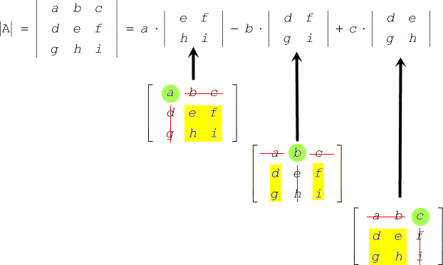
The following video provides an excellent, detailed walkthrough of applying Cramer's rule to a 3x3 system.

For a more formal and comprehensive explanation of both methods, the following reading is recommended.

Consistency of Equations: Unique, Infinite, or No Solution?

A critical part of solving linear systems is determining if a solution even exists and if it's unique. Both methods rely on the determinant of the coefficient matrix, $D=\det (A)$.

1. Unique Solution:
   If $D\ne 0$, the system is consistent and has exactly one unique solution. Both the matrix inversion method and Cramer's rule will work perfectly.

2. No Unique Solution:
   If $D=0$, the matrix $A$ is singular, and its inverse $A^{-1}$ does not exist. The system does not have a unique solution. There are two possibilities in this case:

   • No Solution: The system is inconsistent. The equations contradict each other (e.g., $x+y=2$ and $x+y=3$).
   • Infinitely Many Solutions: The system is consistent but dependent. At least one equation is a combination of the others (e.g., $x+y=2$ and $2x+2y=4$).

Cramer's rule gives us a straightforward way to distinguish between these two cases when $D=0$:

• If $D=0$ and at least one of $D_x,D_y,$ or $D_z$ is non-zero, the system has No Solution.
• If $D=0$ and all of $D_x,D_y,$ and $D_z$ are also zero, the system has Infinitely Many Solutions.

This logic is summarized in the chart below.

For the matrix inversion method, if $\det (A)=0$, you must investigate further. The condition is to check the product $\mathrm{adj}(A)\cdot B$:

• If $\mathrm{adj}(A)\cdot B=0$ (the zero matrix), there are infinitely many solutions.
• If $\mathrm{adj}(A)\cdot B\ne 0$, there is no solution.

Let's read a clear summary of these conditions.

Conclusion

In this lesson, we have equipped ourselves with two robust methods for solving systems of linear equations. The matrix inversion method ($X=A^{-1}B$) leverages our ability to find a matrix inverse and is a direct application of the concepts from our previous session. Cramer's rule provides an elegant, determinant-based alternative that can be particularly efficient if you only need to find one variable.

Crucially, we've also learned how to determine the nature of the solution. The value of the main determinant, $D=\det (A)$, is the primary indicator: if $D\ne 0$, a unique solution is guaranteed. If $D=0$, we must test further to see if there are no solutions or infinitely many, a concept known as checking for consistency.

In our next lesson, we will delve deeper into the properties of matrices and determinants. We'll formalize the ideas of singularity and consistency, exploring how these properties are tested and applied in various problem types you'll encounter in the MHT-CET.