Higher-Order Derivatives

1. What Are Higher-Order Derivatives?

The derivative of a function, $f^{\prime }(x)$, tells us the instantaneous rate of change of $f(x)$. Since $f^{\prime }(x)$ is itself a function, we can differentiate it again. This gives us the second derivative, denoted as $f^{\prime \prime }(x)$. We can continue this process to find the third derivative, $f^{\prime \prime \prime }(x)$, the fourth derivative, and so on. Collectively, these are known as higher-order derivatives.

In physics, if a function $s(t)$ represents an object's position at time $t$, you'll recognize the first derivative, $s^{\prime }(t)$, as its velocity $v(t)$, and the second derivative, $s^{\prime \prime }(t)$, as its acceleration $a(t)$. The third derivative is known as "jerk".

There are two main systems of notation for higher-order derivatives, both of which you need to know.

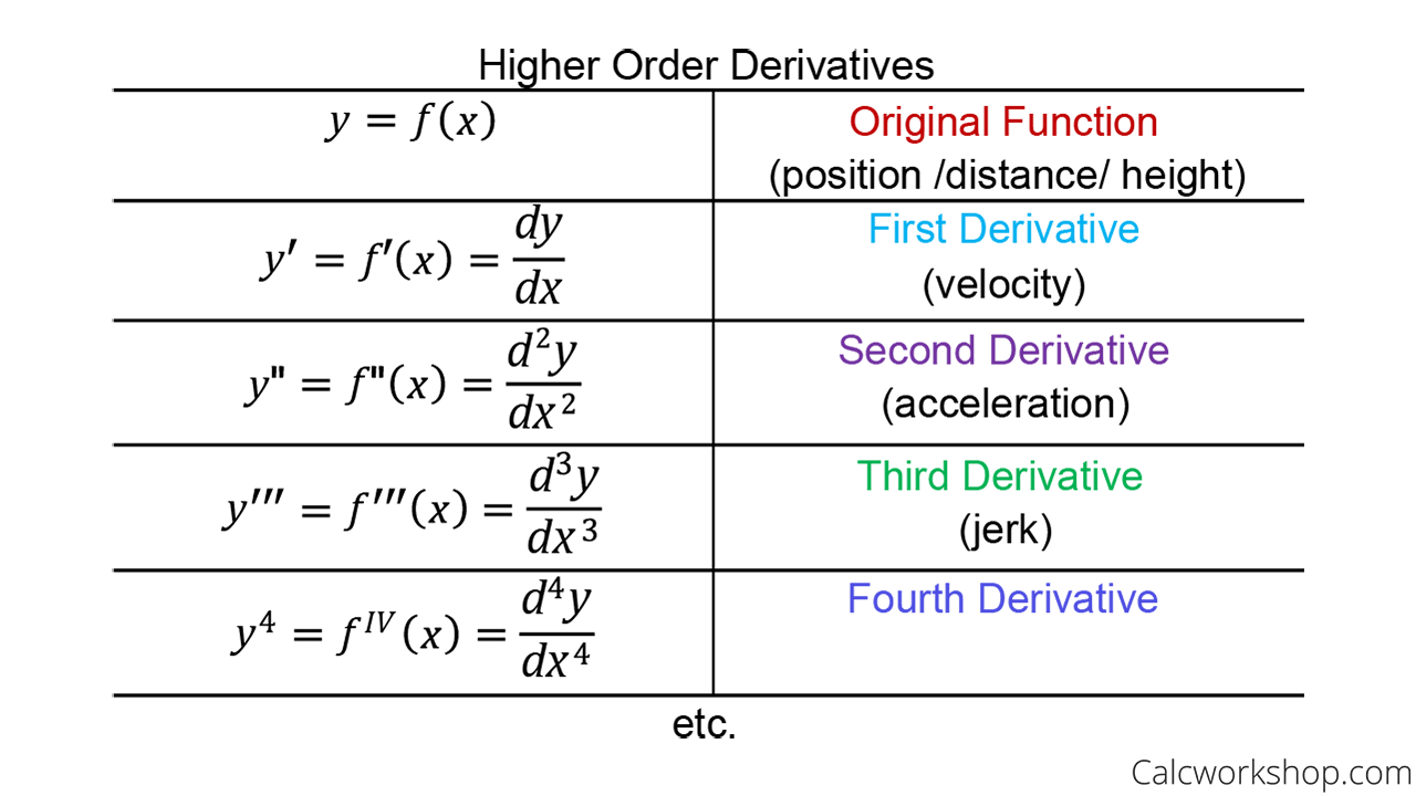
The following resource provides a formal introduction to the concept and notation.

2. Calculating Higher-Order Derivatives

The process of finding higher-order derivatives is straightforward: you simply differentiate again. However, the complexity can increase with each step, sometimes requiring you to use the product or quotient rule for a second derivative even if the first one was simple.

Let's look at some examples.

A crucial fact to remember for polynomials: if $p(x)$ is a polynomial of degree $n$, its $(n+1)$-th derivative will always be zero. For instance, the fourth derivative of $f(x)=5x^3-3x^2+10x-5$ is zero.

3. Second Derivatives of Implicit and Parametric Functions

For your MHT-CET exam, you'll frequently encounter problems requiring second derivatives of functions that aren't simple explicit forms like $y=f(x)$.

Implicit Functions

To find $y^{\prime \prime }$ for an implicit function, you must:

1. Find $y^{\prime }$ using implicit differentiation.
2. Differentiate the expression for $y^{\prime }$ with respect to $x$ again. This will introduce a $y^{\prime }$ term.
3. Substitute the expression for $y^{\prime }$ from step 1 back into your equation for $y^{\prime \prime }$. The final answer for $y^{\prime \prime }$ should be in terms of $x$ and $y$ only.

A key strategy for MHT-CET, especially when finding higher-order derivatives, is to simplify the expression for $y^{\prime }$ before differentiating again.

Parametric Functions

Finding the second derivative for parametric equations is a common source of mistakes. If $x=f(t)$ and $y=g(t)$, we know the first derivative is $\frac{dy}{dx}=\frac{dy/dt}{dx/dt}$.

To find the second derivative, we differentiate $\frac{dy}{dx}$ with respect to $x$. Since $\frac{dy}{dx}$ is a function of $t$, we must use the chain rule:

$\frac{d^{2}y}{d{x}^2}=\frac{d}{dx}\left(\frac{dy}{dx}\right)=\frac{\frac{d}{dt}\left(\frac{dy}{dx}\right)}{\frac{dx}{dt}}$

Crucially, do not forget to divide by $\frac{dx}{dt}$ at the end!

This resource provides a clear derivation and an example.

4. MHT-CET Shortcuts for Second Derivatives

For competitive exams like MHT-CET, recognizing patterns that lead to simple second derivatives can save you a significant amount of time. Many complex-looking functions simplify to have a second derivative of zero.

A key pattern to remember is:
If the first derivative $\frac{dy}{dx}=\frac{y}{x}$, then the second derivative $\frac{d^{2}y}{d{x}^2}$ will always be 0.

Let's see why:
Using the quotient rule, $\frac{d^{2}y}{d{x}^2}=\frac{x\cdot \frac{dy}{dx}-y\cdot 1}{x^2}$.
Substitute $\frac{dy}{dx}=\frac{y}{x}$:
$\frac{d^{2}y}{d{x}^2}=\frac{x\cdot (\frac{y}{x})-y}{x^2}=\frac{y-y}{x^2}=0$

The trick is to identify functions where $\frac{dy}{dx}=\frac{y}{x}$. The following video covers two major types.

Memorizing these patterns will allow you to answer certain higher-order derivative questions in seconds.

Conclusion

In this lesson, you've learned how to find derivatives beyond the first order. This is a fundamental skill that builds directly on all the differentiation rules you already know.

Key Takeaways:

• Higher-order derivatives are found by differentiating a function repeatedly.
• You must be familiar with both prime notation ($f^{\prime \prime },f^{\prime \prime \prime }$) and Leibniz notation ($\frac{d^{2}y}{d{x}^2},\frac{d^{3}y}{d{x}^3}$).
• To find $y^{\prime \prime }$ for implicit functions, differentiate $y^{\prime }$ and substitute the expression for $y^{\prime }$ back in.
• For parametric functions, the second derivative is $\frac{d^{2}y}{d{x}^2}=\frac{d/dt(dy/dx)}{dx/dt}$.
• For MHT-CET, look for shortcuts where $\frac{dy}{dx}=\frac{y}{x}$, as this immediately implies $\frac{d^{2}y}{d{x}^2}=0$.

In our next lesson, we will begin applying our knowledge of derivatives. We'll focus on the learning outcome: Find equations of tangents and normals to a curve at a given point. This will be our first step into using derivatives to analyze the geometric properties of functions.