Gradients and Hessians of Multivariable Functions

Welcome to the first lesson of your course on Statistical Machine Learning. We'll begin by building a solid mathematical foundation, which will be indispensable as we move into more complex models and algorithms. This initial module focuses on the tools of multivariate calculus and optimisation that form the bedrock of modern machine learning.

Today's lesson addresses a core concept: computing derivatives for functions with multiple inputs. You'll learn how to calculate the gradient and the Hessian matrix for scalar-valued functions. In machine learning, we often define a "loss" or "cost" function that measures how poorly our model is performing. This is a scalar value that depends on many parameters. The gradient tells us the direction to adjust these parameters to improve the model, while the Hessian gives us information about the shape of the loss landscape, helping us understand if we've found a true minimum.

1. From Derivatives to Partial Derivatives and Gradients

You're familiar with the derivative of a function of a single variable, $f (x)$ , which gives the slope of the function at a point. But what happens when a function has multiple inputs, like $f (x, y)$ ? The rate of change depends on which direction we move.

The simplest way to approach this is to see how the function changes as we vary one input at a time, holding the others constant. This leads to the idea of partial derivatives.

To get a formal introduction, please read the following section from the article "The Matrix Calculus You Need For Deep Learning". It clearly explains how to compute partial derivatives and how they are assembled into a vector called the gradient.

The Matrix Calculus You Need For Deep Learning

This reading introduces the core idea of partial derivatives and the gradient.

Please read the section titled "Introduction to vector calculus and partial derivatives". Focus on understanding how a partial derivative, like \frac{\partial f}{\partial x}, is calculated by treating other variables (like y) as constants. Pay close attention to how the gradient, \nabla f, is defined as a vector containing all the partial derivatives.

The key idea is that the gradient, $\nabla f$ , packages all the first-order derivative information into a single vector. For a function $f (x)$ where $x = (x_{1}, x_{2}, \dots, x_{n})$ is a vector of variables, the gradient is:

\nabla f (x) = \frac{\partial f}{\partial x _{1}} \frac{\partial f}{\partial x _{2}} ⋮ \frac{\partial f}{\partial x _{n}}

Geometrically, the gradient vector at a point $x$ points in the direction of the steepest ascent of the function. Its magnitude represents the rate of increase in that direction. In machine learning, we will often move in the opposite direction of the gradient to minimize a loss function—this is the core idea of gradient descent.

To see this in action and practice your calculations, please watch the following video. It provides clear, step-by-step examples. I encourage you to pause the video and try the calculations yourself.

How To Find The Directional Derivative and The Gradient Vector

This video from The Organic Chemistry Tutor demonstrates how to compute the components of the gradient vector and assemble it for functions of two and three variables.

Watch the two segments below. The first works through a 2D example, and the second tackles a 3D one. 2D Example: Watch from this segment to see how to find the gradient of f(x, y) and evaluate it at a point. 3D Example: Now watch the segment from this example, which extends the concept to a function f(x, y, z).

2. The Hessian: Curvature and Second Derivatives

Now that we have the first derivative (the gradient), let's move on to the second derivative. For a single-variable function, the second derivative $f^{''} (x)$ tells us about the function's curvature (whether it's concave up or down). For a multivariable function, this role is played by the Hessian matrix, denoted $H$ .

The Hessian is the matrix of all possible second-order partial derivatives. If the gradient is the derivative of a scalar function $f$ , the Hessian can be thought of as the "derivative of the gradient".

The following reading from an MIT course provides a formal definition.

Second Derivatives, Bilinear Maps, and Hessian Matrices

This resource defines the Hessian matrix and clarifies its properties.

First, read the section "Hessian matrices of scalar-valued functions" on page 87. This introduces the Hessian as the Jacobian of the gradient. Note the definition of its entries: H_{i,j} = \frac{\partial^2 f}{\partial x_j \partial x_i}. Then, on page 88, read Remark 54, which highlights the key distinction between a general Jacobian matrix and the specific case of the Hessian, which is always square and symmetric.

For a function $f (x_{1}, \dots, x_{n})$ , the Hessian matrix is an $n \times n$ matrix defined as:

H = \frac{\partial ^{2} f}{\partial x _{1}^{2}} \frac{\partial ^{2} f}{\partial x _{2} \partial x _{1}} ⋮ \frac{\partial ^{2} f}{\partial x _{n} \partial x _{1}} \frac{\partial ^{2} f}{\partial x _{1} \partial x _{2}} \frac{\partial ^{2} f}{\partial x _{2}^{2}} ⋮ \frac{\partial ^{2} f}{\partial x _{n} \partial x _{2}} \dots \dots ⋱ \dots \frac{\partial ^{2} f}{\partial x _{1} \partial x _{n}} \frac{\partial ^{2} f}{\partial x _{2} \partial x _{n}} ⋮ \frac{\partial ^{2} f}{\partial x _{n}^{2}}

A crucial property, as mentioned in the reading, is that the Hessian is symmetric, meaning $H = H^{T}$ . This is because for most well-behaved functions (which are common in machine learning), the order of partial differentiation does not matter (e.g., $\frac{\partial ^{2} f}{\partial x _{1} \partial x _{2}} = \frac{\partial ^{2} f}{\partial x _{2} \partial x _{1}}$ ). This is known as Clairaut's theorem or the equality of mixed partials.

Example Calculation

Let's compute the Hessian for $f (x, y) = x^{2} y^{3} + e^{2 x}$ .

First Partial Derivatives (Gradient components):
- $\frac{\partial f}{\partial x} = 2 x y^{3} + 2 e^{2 x}$
- $\frac{\partial f}{\partial y} = 3 x^{2} y^{2}$
Second Partial Derivatives (Hessian components):
- $\frac{\partial ^{2} f}{\partial x ^{2}} = \frac{\partial}{\partial x} (2 x y^{3} + 2 e^{2 x}) = 2 y^{3} + 4 e^{2 x}$
- $\frac{\partial ^{2} f}{\partial y ^{2}} = \frac{\partial}{\partial y} (3 x^{2} y^{2}) = 6 x^{2} y$
- $\frac{\partial ^{2} f}{\partial y \partial x} = \frac{\partial}{\partial y} (2 x y^{3} + 2 e^{2 x}) = 6 x y^{2}$
- $\frac{\partial ^{2} f}{\partial x \partial y} = \frac{\partial}{\partial x} (3 x^{2} y^{2}) = 6 x y^{2}$ (Note that these are equal, as expected!)
Assemble the Hessian Matrix:
$H = (2 y^{3} + 4 e^{2 x} 6 x y^{2} 6 x y^{2} 6 x^{2} y)$

A particularly important function in machine learning is the quadratic form $f (x) = x^{T} A x$ . It appears in linear regression, support vector machines, and many other areas. Let's see how to compute its Hessian.

Second Derivatives, Bilinear Maps, and Hessian Matrices

This example is a fundamental result in matrix calculus for machine learning.

On page 91, read through Example 58. It shows the derivation for the Hessian of f(\mathbf{x}) = \mathbf{x}^T A \mathbf{x}. Given your comfort with matrix operations, this derivation should be quite approachable. The result is surprisingly simple: H = A + A^T. If A is symmetric, the Hessian is simply 2A.

3. Interpreting the Hessian: The Second Derivative Test

Why is the Hessian so important? At a point where the gradient is zero ( $\nabla f = 0$ ), called a critical point, the Hessian tells us the "shape" of the function. This allows us to classify the point as a local minimum, local maximum, or a saddle point.

This is analogous to the second derivative test from single-variable calculus:

If $f^{'} (x_{0}) = 0$ and $f^{''} (x_{0}) > 0$ , then $x_{0}$ is a local minimum.
If $f^{'} (x_{0}) = 0$ and $f^{''} (x_{0}) < 0$ , then $x_{0}$ is a local maximum.

For multiple variables, the sign of the Hessian is replaced by its definiteness, which is determined by the signs of its eigenvalues.

The following image provides a fantastic visual intuition for this concept.

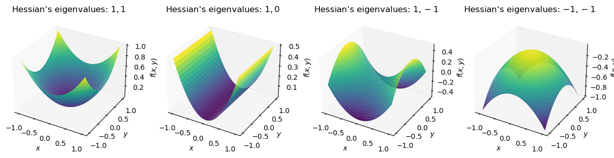
These plots show how the shape of a function $f(x, y)$ around a critical point is determined by the eigenvalues of its Hessian matrix at that point. From left to right: local minimum, a "valley" or flat direction, a saddle point, and a local maximum.

Let's break down the connection:

Local Minimum (top-left plot): The function curves upwards in all directions, like a bowl. This happens when the Hessian is positive-definite, meaning all its eigenvalues are positive ( $λ_{1} > 0, λ_{2} > 0$ ).
Local Maximum (bottom-right plot): The function curves downwards in all directions, like a dome. This corresponds to a negative-definite Hessian, where all eigenvalues are negative ( $λ_{1} < 0, λ_{2} < 0$ ).
Saddle Point (top-right plot): The function curves up in one direction and down in another, like a saddle. The Hessian is indefinite, with both positive and negative eigenvalues ( $λ_{1} > 0, λ_{2} < 0$ ).
Degenerate Case (bottom-left plot): One direction is curved, but another is flat. The Hessian is positive semi-definite (or negative semi-definite), with at least one eigenvalue being zero ( $λ_{1} > 0, λ_{2} = 0$ ). These points are common in deep learning and can lead to plateaus where training slows down.

The following text formalizes this relationship.

Second Derivatives, Bilinear Maps, and Hessian Matrices

This section summarizes the "second derivative test" for multivariable functions.

On page 93, read the subsection "Minima, maxima, and saddle points". Focus on the conditions for a local minimum and maximum based on the definiteness of the Hessian and the signs of its eigenvalues.

Conclusion

In this lesson, we have laid the groundwork for the calculus of optimisation in machine learning. You've learned to compute and interpret the two most important derivatives for scalar-valued functions.

Here are the key takeaways:

The gradient ( $\nabla f$ ) is a vector of first partial derivatives. It points in the direction of the function's steepest ascent and is fundamental to optimisation algorithms like gradient descent.
The Hessian ( $H$ ) is a symmetric matrix of second partial derivatives. It describes the local curvature of a function.
At a critical point (where $\nabla f = 0$ ), the eigenvalues of the Hessian determine the nature of that point: a local minimum (all positive eigenvalues), a local maximum (all negative eigenvalues), or a saddle point (mixed signs).

In our next lesson, we will generalise these ideas to vector-valued functions by introducing the Jacobian matrix. We will then explore the multivariate chain rule, a powerful tool that forms the basis of the backpropagation algorithm used to train neural networks.

Recommended resources

1. From Derivatives to Partial Derivatives and Gradients

2. The Hessian: Curvature and Second Derivatives

Example Calculation

3. Interpreting the Hessian: The Second Derivative Test

Conclusion