Vanilla Gradient Descent for Convex Functions

Hello! In our previous lesson, we mastered the method of Lagrange multipliers, a powerful analytical tool for solving constrained optimisation problems. This method is elegant when we can algebraically solve the system of equations it produces. However, in many complex machine learning scenarios, finding such a direct solution for where a gradient is zero is either computationally infeasible or mathematically impossible.

This lesson introduces an essential alternative: an iterative, algorithmic approach. We will explore gradient descent, arguably the most fundamental optimisation algorithm in machine learning. Instead of solving for the optimal parameters in one go, we will learn how to "walk" towards them step-by-step. This lesson directly addresses your goal of becoming comfortable with gradient descent.

Our learning objective is to implement vanilla gradient descent to minimise a convex function. We will do this in a hands-on way that aligns with your preference for active learning. You'll write the code to train a simple linear regression model from scratch, giving you a concrete and foundational understanding of how modern machine learning models are trained.

1. The Core Idea: Walking Down the Loss Landscape

Imagine you are on a foggy mountain and want to get to the lowest valley. You can't see the entire landscape, but you can feel the slope of the ground right where you are standing. The most straightforward strategy would be to take a step in the direction of the steepest descent. You'd repeat this process, and each step would take you to a lower altitude, until you eventually reach the bottom.

This is the exact intuition behind gradient descent. In machine learning, the "mountain" is our loss function (also called a cost function), $J (θ)$ , which measures how poorly our model is performing. The "location" on the mountain is the current set of our model's parameters, $θ$ . The "slope" is given by the gradient of the loss function, $\nabla J (θ)$ . Since the gradient points in the direction of the steepest ascent, we move in the direction of the negative gradient to go downhill.

This process is captured by a simple iterative update rule:

θ_{n e w} = θ_{o l d} - η \nabla J (θ_{o l d})

Let's break this down:

$θ_{o l d}$ is our current set of parameters.
$\nabla J (θ_{o l d})$ is the gradient of the loss function evaluated at our current parameters. It tells us the direction of steepest ascent.
$η$ (eta) is the learning rate, a small positive number that controls how large of a step we take.
$θ_{n e w}$ is our updated set of parameters, which should correspond to a lower point on the loss function.

We repeat this update until we converge to a minimum.

The following video from StatQuest provides an excellent conceptual overview of this entire process.

Gradient Descent, Step-by-Step

This video from StatQuest with Josh Starmer gives a clear, step-by-step walkthrough of the gradient descent algorithm in the context of linear regression.

Please watch these two segments: First, watch the introduction from the beginning to understand the role of optimisation in machine learning. Then, watch from this point to see the core iterative process explained: calculating the slope (gradient), determining the step size with a learning rate, and updating the parameter.

2. A Concrete Problem: Simple Linear Regression

To implement gradient descent, we need a function to minimise. Let's use a simple but practical machine learning problem: fitting a line to some data. We'll use a model with just one parameter, the slope w, assuming the line passes through the origin:

y = w \cdot x

Our goal is to find the value of $w$ that makes this line fit our data best. To measure the "fit", we'll use the Mean Squared Error (MSE) loss function. This function calculates the average of the squared differences between the true target values ( $t_{i}$ ) and our model's predictions ( $y_{i}$ ).

J (w) = \frac{1}{N} i = 1 \sum N (t_{i} - y_{i})^{2} = \frac{1}{N} i = 1 \sum N (t_{i} - w \cdot x_{i})^{2}

A crucial property of the MSE loss for linear regression is that it is a convex function with respect to the parameter $w$ . As we learned in a previous lesson, this guarantees that there is only one minimum, which is the global minimum. This means gradient descent won't get stuck in a suboptimal local minimum.

For a convex function (left), any local minimum is also the global minimum. For a non-convex function (right), gradient descent might get stuck in a local minimum instead of finding the global one.

The following resource will guide us through setting up this problem, from generating synthetic data to defining the model and loss function in Python.

How to implement a neural network (1/5) - gradient descent

This article by Peter Roelants provides a complete, self-contained example of using gradient descent for linear regression. It's perfect for our goal of a hands-on implementation.

Please read the first three sections of the article. Start with the problem setup to understand the simple model we're using. Next, review the data generation section to see how the toy dataset is created. You can skim the Python code here for now; we'll focus on it more later. Finally, read the section defining the loss function. Pay close attention to the plot of the loss function versus the weight w. Notice its parabolic (convex) shape.

3. Deriving the Gradient

Our update rule requires the gradient of the loss function, $\frac{\partial J}{\partial w}$ . We need to calculate how the MSE loss changes as we change the weight $w$ . We can find this derivative using the chain rule.

For a single data point $i$ , the loss is $(t_{i} - w \cdot x_{i})^{2}$ . Its derivative with respect to $w$ is:

\frac{\partial J _{i}}{\partial w} = \frac{\partial ( t _{i} - w \cdot x _{i} ) ^{2}}{\partial w} = 2 (t_{i} - w \cdot x_{i}) \cdot (- x_{i}) = - 2 x_{i} (t_{i} - y_{i})

For the total MSE loss, we average this over all $N$ data points:

\frac{\partial J}{\partial w} = \frac{1}{N} i = 1 \sum N - 2 x_{i} (t_{i} - y_{i}) = \frac{2}{N} i = 1 \sum N x_{i} (y_{i} - t_{i})

This is the formula we'll need to implement. It tells us the slope of our loss function at our current position $w$ , which we then use to update our position.

4. Implementing Gradient Descent in Python

Now we have all the pieces: the model, the loss function, and the gradient. Let's put them together in Python. This is a great opportunity for you to open a code editor and "write things down" as we go. We'll follow the clear structure provided in the Peter's Notes article.

How to implement a neural network (1/5) - gradient descent

This section of the article walks through the derivation and implementation of the gradient descent update.

First, read the subsection Gradient descent, which shows the derivation we just discussed. Next, carefully study the Python code in the following section. This is where we translate the math into a working algorithm. Pay attention to these parts of the code block under In [6]: The gradient(w, x, t) function, which implements our derived gradient formula. The delta_w(...) function, which calculates the full update step (\eta \cdot \nabla J). The for loop, which performs the iterative updates. Notice how w is updated in each iteration: w = w - dw.

To see a live demonstration of this coding process, the following video is highly recommended. It builds a very similar implementation from scratch, which can help solidify your understanding.

Gradient Descent From Scratch in Python - Visual Explanation

This video by NeuralNine provides an excellent, intuitive, and from-scratch implementation of gradient descent in Python.

Watching someone code this live can be very helpful. First, watch the conceptual explanation which uses a simple drawing to build intuition. Then, follow the coding segment where the presenter implements gradient descent for a simple x^2 function. The logic is identical to our linear regression problem: define a function, define its derivative, and write an update loop with a learning rate.

5. The Crucial Role of the Learning Rate

As you've seen in the code and update rule, the learning rate $η$ is a critical hyperparameter. It determines the size of the steps we take down the loss function.

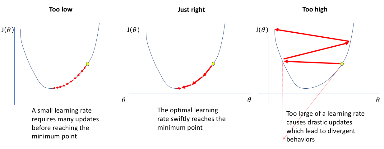
Too low: If $η$ is too small, we will take tiny steps, and the algorithm will converge very slowly. It might take an impractically long time to reach the minimum.
Too high: If $η$ is too large, we might overshoot the minimum entirely. The steps are so big that we jump from one side of the valley to the other, and the loss might oscillate or even diverge, increasing with every step.
Just right: An appropriate learning rate ensures we converge to the minimum in a reasonable number of steps.

The image below illustrates these three scenarios perfectly.

The choice of learning rate is critical for the convergence of gradient descent. A low rate leads to slow convergence, a high rate can lead to divergence, while an optimal rate leads to fast convergence.

The videos and articles you've looked at also touch on this. In particular, the NeuralNine video has a great demonstration of changing the learning rate and seeing the effect live.

Conclusion

In this lesson, we have demystified one of the most important algorithms in machine learning. We moved from the world of analytical solutions to the practical, iterative approach that powers the training of large-scale models.

Here are the key takeaways:

Gradient Descent is an iterative optimisation algorithm that finds the minimum of a function by repeatedly taking steps in the direction of the negative gradient.
The core of the algorithm is the update rule: $θ_{n e w} = θ_{o l d} - η \nabla J (θ_{o l d})$ .
We implemented this algorithm from scratch for a simple linear regression model, using the Mean Squared Error as our convex loss function.
The learning rate ( $η$ ) is a critical hyperparameter that controls the step size and dramatically affects the algorithm's convergence.

We've seen visually how the learning rate can make or break the optimisation process. In our next lesson, we will formalise this understanding by analysing the effect of the learning rate on gradient descent convergence more rigorously and exploring some practical strategies for setting this important parameter.