Large Deviations and the Emergence of Thermodynamic Potentials

Welcome back. In our last lesson, we established a crucial quantitative result: in the thermodynamic limit, the relative fluctuations of extensive quantities like energy scale as $1/ N$ , becoming negligible for macroscopic systems. This provided the mathematical backbone for the concept of ensemble equivalence. We saw that for a system in the canonical ensemble, its energy distribution is incredibly sharp, making it almost indistinguishable from a system with a fixed energy in the microcanonical ensemble.

This naturally leads to a deeper question. We understand that macroscopic deviations from the average are rare, but how rare? What is the probability of observing a system spontaneously fluctuate to an energy, volume, or particle number far from its equilibrium value? The Central Limit Theorem describes the small, Gaussian fluctuations around the mean, but it cannot answer this question. To do so, we must turn to the theory of large deviations.

Today's lesson aims to apply the large deviation principle to show how the canonical and grand canonical potentials emerge as rate functions governing macroscopic fluctuations away from the microcanonical state. By the end of our session, you will understand how thermodynamic potentials like the Helmholtz and Gibbs free energies are not just convenient calculational tools, but are in fact the very functions that quantify the exponential improbability of observing a system in a non-equilibrium macrostate. This will provide our most profound perspective yet on the connection between ensembles and the principles of maximum entropy and minimum free energy.

1. The Large Deviation Principle: A Visual and Formal Introduction

At its heart, the theory of large deviations provides an asymptotic estimate for the probability of rare events. Imagine we are repeatedly measuring some averaged quantity, like the energy per particle $h_{N} = E / N$ of a system of $N$ particles. The law of large numbers tells us that as $N \to \infty$ , this value will converge to a specific average, $⟨ h ⟩$ . Large deviation theory tells us how the probability of observing a different value, $h_{N} = u$ , behaves for large $N$ .

The central statement is the Large Deviation Principle (LDP). It posits that for large $N$ , the probability distribution has an exponential form:

P (h_{N} = u) \approx e^{- N I (u)}

The key components here are:

The speed of the decay, which is the scaling parameter $N$ .
The rate function $I (u)$ , a non-negative function ( $I (u) \geq 0$ ) that quantifies the improbability of observing the value $u$ .

A crucial property of the rate function is that it is zero only at the most probable value, $I (⟨ h ⟩) = 0$ , and positive everywhere else. This means the probability of observing any value other than the average decays exponentially to zero as $N$ increases. This exponential suppression is the essence of why we observe stable thermodynamic states macroscopically.

The following image provides a powerful visual summary of these ideas.

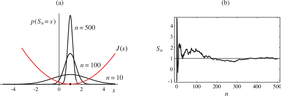
Figure 1. (a) The probability distribution $p(S_n=s)$ for an averaged quantity $S_n$ becomes increasingly peaked as the system size $n$ grows, concentrating at the value where the rate function $J(s)$ is zero. (b) A single realization of the process, showing the convergence of the average $S_n$ to its mean value.

To formalize this, the rate function is defined by the limit:

I (u) = N \to \infty lim - \frac{1}{N} ln P (h_{N} = u)

This definition provides a way to calculate $I (u)$ if we know the probability distribution. However, it is often easier to calculate it via its Legendre transform.

To see this connection, watch the following video segment. It provides a clear, conceptual introduction to the Large Deviation Principle, the rate function, and the powerful Gärtner-Ellis Theorem that connects the rate function to a quantity we can often calculate: the scaled cumulant generating function (SCGF).

Large deviations of Markov processes (Part - 1) by Hugo Touchette

This excerpt from a lecture by Prof. Hugo Touchette, a leading expert in the field, introduces the core ideas of large deviation theory in an accessible way.

First, watch the segment that defines the Large Deviation Principle and the properties of the rate function. Notice how the LDP describes the exponential concentration of the probability distribution. Then, continue with the introduction of the Gärtner-Ellis theorem, which establishes the Legendre transform relationship between the rate function I(a) and the scaled cumulant generating function \lambda(k).

As the video explains, the Gärtner-Ellis Theorem is a cornerstone of LDT. It states that if the following limit, called the Scaled Cumulant Generating Function (SCGF), exists and is differentiable:

λ (k) = N \to \infty lim \frac{1}{N} ln ⟨ e^{N k h_{N}} ⟩

then the rate function is its Legendre-Fenchel transform:

I (u) = k \in R sup {k u - λ (k)}

This is a powerful result because, as we will now see, the SCGF $λ (k)$ is directly related to thermodynamic potentials.

2. From Large Deviations to Thermodynamics

Let's apply this formalism to equilibrium statistical mechanics. We will start from the most fundamental level—the microcanonical ensemble—and see how the canonical free energy emerges naturally from large deviation theory.

For a deeper and more rigorous treatment of the ideas we'll discuss, the following text is an invaluable resource.

1 Large deviation approach to nonequilibrium systems

This chapter, also by Hugo Touchette, provides the rigorous mathematical framework connecting LDT and statistical mechanics.

Begin by reading the section "Equilibrium systems" (pp. 2-5). This section formalizes the idea of "typicality" and explains why intensive quantities like energy per particle are the correct macroscopic variables to consider, as they are the ones whose distributions concentrate. Next, read the section "Equilibrium large deviations" (pp. 9-12). This is the core of our lesson. Follow the argument that connects the entropy, free energy, and the Legendre transform structure of thermodynamics to the LDP for the energy density.

Let's unpack the argument presented in the reading.

1. Entropy as a Rate Function (in disguise)

Consider an isolated system with Hamiltonian $H_{N}$ . The fundamental postulate states that all accessible microstates are equally likely. We are interested in the probability of observing the energy per particle, $h_{N} = H_{N} / N$ , to have a value $u$ . This probability is proportional to the number of microstates with that energy, i.e., the density of states $Ω (E = N u)$ .

P (h_{N} = u) \propto Ω (N u)

From our definition of Boltzmann entropy, $S (E) = k_{B} ln Ω (E)$ . For a macroscopic system, entropy is extensive, so $S (E = N u) \approx N s (u)$ , where $s (u)$ is the entropy per particle. Therefore,

P (h_{N} = u) \approx e^{N s (u) / k_{B}}

Comparing this to the LDP form $P (h_{N} = u) \approx e^{- N I (u)}$ , we see a direct correspondence:

I (u) = - s (u) / k_{B}

Here, the entropy $s (u)$ acts as a rate function, but with a negative sign. This is because we are considering the probability of any state, and states with higher entropy are more probable. Large deviation theory is usually framed for probabilities that decay, so we identify the rate of decay with $- s (u)$ .

2. Free Energy as the SCGF

Now, let's compute the SCGF, $λ (k)$ , for the energy density $h_{N}$ under the same uniform measure.

λ (k) = N \to \infty lim \frac{1}{N} ln ⟨ e^{N k h_{N}} ⟩ = N \to \infty lim \frac{1}{N} ln (microstates \sum e^{k H_{N}}) - const.

The summation term is precisely the canonical partition function $Z_{N}$ if we identify the parameter $k$ with $- β = - 1/ (k_{B} T)$ . Let's do that: $k = - β$ .

λ (- β) = N \to \infty lim \frac{1}{N} ln Z_{N} (β)

Recalling the definition of the Helmholtz free energy, $F = - k_{B} T ln Z$ , or $ln Z = - β F$ , we can relate the SCGF to the free energy per particle, $f (β) = lim F_{N} / N$ .

λ (- β) = N \to \infty lim \frac{- β F _{N} ( β )}{N} = - β f (β)

The SCGF is simply the (negative, scaled) free energy per particle.

3. The Legendre Transform Connection

The Gärtner-Ellis theorem tells us $I (u) = sup_{k} {k u - λ (k)}$ . Substituting our expressions for $I (u)$ and $λ (k)$ :

- s (u) / k_{B} = - β sup {- β u - λ (- β)} = - β sup {- β u - (- β f (β))}

- s (u) / k_{B} = - β sup {- β (u - f (β))}

Taking the $k_{B}$ over and flipping the supremum to an infimum by changing the sign:

s (u) = β in f {β k_{B} (u - f (β))} = T in f {\frac{u - f ( T )}{T}}

This is exactly the Legendre transform that connects entropy and free energy in thermodynamics! Large deviation theory provides a probabilistic foundation for this fundamental structure.

3. Thermodynamic Potentials as Fluctuation Rate Functions

We have just seen how, starting from the microcanonical viewpoint, the canonical free energy naturally emerges as the Legendre transform of the entropy. Now we will flip the perspective. Let's assume our system is in contact with a heat bath at a fixed temperature $T$ (i.e., it is in the canonical ensemble) and ask: what is the probability that its energy density spontaneously fluctuates to a value $u$ different from the equilibrium average $⟨ h ⟩_{β}$ ?

The LDP states that this probability is $P_{β} (h_{N} = u) \approx e^{- N I_{β} (u)}$ , where $I_{β} (u)$ is the rate function for fluctuations within the canonical ensemble. Let's find this rate function.

The probability of observing a system with energy $N u$ in the canonical ensemble is:

P_{β} (h_{N} = u) = \frac{Ω ( N u ) e ^{- β N u}}{Z _{N} ( β )}

Taking the logarithm, dividing by $- N$ , and taking the limit $N \to \infty$ :

I_{β} (u) = N \to \infty lim - \frac{1}{N} [ln Ω (N u) - β N u - ln Z_{N} (β)]

Using our previous identifications, $lim \frac{1}{N} ln Ω (N u) = s (u) / k_{B}$ and $lim \frac{1}{N} ln Z_{N} (β) = - β f (β)$ , we get:

I_{β} (u) = - (\frac{s ( u )}{k _{B}} - β u + β f (β))

Rearranging this using $β = 1/ (k_{B} T)$ gives:

I_{β} (u) = β ((u - T s (u)) - f (β))

We recognize the term $u - T s (u)$ as the Helmholtz free energy corresponding to the macrostate with energy $u$ , let's call it $f (u)$ . The term $f (β)$ is the equilibrium free energy at the temperature $T = 1/ (k_{B} β)$ of the bath. So we have our main result:

I_{β} (u) = β [f (u) - f (β)] = \frac{f ( u ) - f _{e q}}{k _{B} T}

This remarkable equation states that the rate function—which governs the exponential probability of an energy fluctuation—is simply the difference between the free energy of the fluctuated state and the equilibrium free energy, scaled by $k_{B} T$ .

The minimum free energy principle is now seen in a new light. The probability of observing a state $u$ is $P_{β} (h_{N} = u) \approx e^{- N β [f (u) - f_{e q}]}$ . This probability is maximized when the exponent is minimized, which occurs when $f (u)$ is at its minimum value, $f_{e q}$ . Thus, the equilibrium state is not just the one with the lowest free energy; it is the overwhelmingly most probable state, with all other states being exponentially suppressed.

The same logic applies to the grand canonical ensemble. If we consider a system in contact with a heat and particle reservoir ( $T, μ$ ), the probability of observing a simultaneous fluctuation to energy density $u$ and particle density $ρ$ is governed by a rate function:

I_{β, μ} (u, ρ) = β [Φ (u, ρ) - Φ (β, μ)] = \frac{Φ ( u , ρ ) - Φ _{e q}}{k _{B} T}

Here, $Φ (u, ρ) = u - T s (u, ρ) - μ ρ$ is the grand potential of the fluctuated state, and $Φ_{e q}$ is its equilibrium value. The grand potential directly governs the probability of joint energy and particle number fluctuations.

For a deeper dive into these ideas, particularly how these rate functions are derived using various LDT tools like the contraction principle (used to derive Cramér's theorem from Sanov's) and Varadhan's theorem, you may find the following text insightful.

[PDF] Entropy and Large Deviations Part 1: Classical Theory - Mathematics

This text provides a more mathematical but highly rewarding perspective on these concepts.

You can explore the sections on Sanov's Theorem (pp. 22-24), which gives the LDP for the empirical measure with relative entropy as the rate function, and Cramér's Theorem (pp. 28-29), which gives the LDP for sums of random variables (like energy). The connection between them via the contraction principle is explained in the proof of Theorem 5.2 (p. 33). Lastly, explore the section on General Theory (pp. 37-39), which introduces the contraction principle and Varadhan's theorem, powerful methods for deriving new LDPs.

Conclusion

In this lesson, we have taken a significant step in formalizing the foundations of statistical mechanics, moving beyond the behavior of typical fluctuations to quantify the probability of rare, large ones.

Key Takeaways:

The Large Deviation Principle (LDP) states that the probability of a macroscopic observable deviating from its mean value decays exponentially with system size, $P (h_{N} = u) \approx e^{- N I (u)}$ .
The rate function $I (u)$ quantifies this decay. It is non-negative and is zero only at the equilibrium value.
By applying the LDP to an isolated system, we showed that the Helmholtz free energy emerges as the Legendre transform of the entropy, revealing the probabilistic origin of this core thermodynamic relationship.
Most importantly, for a system in a thermal bath (canonical ensemble), the rate function governing energy fluctuations is directly proportional to the change in the Helmholtz free energy: $I_{β} (u) \propto f (u) - f_{e q}$ .
Similarly, for a system open to heat and particle exchange (grand canonical ensemble), the grand potential acts as the rate function for joint energy and particle number fluctuations.
These results provide the deepest justification for the minimum free energy principle and the equivalence of ensembles. Equilibrium states are not merely the ones with the lowest potential; they are the states where the system resides with a probability that approaches one, while all other macroscopic states are exponentially improbable.

In our next lesson, we will pivot from these abstract principles to a cornerstone application. We will derive the Sackur-Tetrode equation for the entropy of a classical ideal gas. This will allow us to confront a famous puzzle—the Gibbs paradox—and see how a semi-classical correction involving Planck's constant, motivated by the phase space concepts we have discussed, resolves it.

Recommended resources

1. The Large Deviation Principle: A Visual and Formal Introduction

2. From Large Deviations to Thermodynamics

3. Thermodynamic Potentials as Fluctuation Rate Functions

Conclusion