Quantum Partition Functions: Tracing the Statistical Operator

Welcome back. In our previous lesson, we constructed the density operators for the main statistical ensembles by maximizing the von Neumann entropy subject to macroscopic constraints. We found that the canonical density operator, for instance, takes the form $ρ^_{c} = e^{- β H^} / Z$ , where we identified the partition function $Z$ as a normalization constant.

Today, we will formalize this connection and elevate the partition function from a simple normalization factor to the central object from which all equilibrium thermodynamic properties can be derived. The learning outcome for this lesson is to express quantum partition functions as traces of the corresponding statistical operator. We will solidify the definition of the canonical and grand canonical partition functions in this operator language and work through a cornerstone example to see this formalism in action.

1. The Partition Function as a Trace

The trace of an operator, denoted $Tr (A^)$ , is a fundamental concept in linear algebra that you are well-acquainted with. It is defined as the sum of the diagonal elements of the operator's matrix representation in any complete orthonormal basis ${∣ n ⟩}$ :

Tr (A^) = n \sum ⟨ n ∣ A^∣ n ⟩

A crucial property of the trace is its basis-invariance. The value of $Tr (A^)$ is independent of the basis chosen to compute it. This mathematical robustness is what allows the trace to represent a physical quantity, which cannot depend on our arbitrary choice of basis states.

In the last lesson, we derived the canonical density operator:

ρ^_{c} = \frac{e ^{- β H^}}{Z}

The normalization condition, $Tr (ρ^_{c}) = 1$ , immediately provides the formal definition for the canonical partition function, $Z$ :

Tr (\frac{e ^{- β H^}}{Z}) = \frac{1}{Z} Tr (e^{- β H^}) = 1 ⟹ Z = Tr (e^{- β H^})

This is the fundamental quantum mechanical definition. It connects the microscopic physics, encapsulated in the Hamiltonian operator $H^$ , to a single scalar function $Z (β)$ .

To see how this operator definition relates to the sum-over-states formula you've likely used before, we can evaluate the trace in the most convenient basis: the eigenbasis of the Hamiltonian itself. Let ${∣ k ⟩}$ be the set of energy eigenstates, such that $H^∣ k ⟩ = E_{k} ∣ k ⟩$ . Then:

Z = k \sum ⟨ k ∣ e^{- β H^} ∣ k ⟩ = k \sum e^{- β E_{k}} ⟨ k ∣ k ⟩ = k \sum e^{- β E_{k}}

This confirms that the formal trace definition correctly reduces to the familiar sum of Boltzmann factors over all quantum states of the system.

The following resources provide a concise statement of this central definition.

[PDF] Statistical Mechanics I - MIT OpenCourseWare

These lecture notes by Mehran Kardar provide a rigorous path from the axioms of quantum mechanics to the ensembles of statistical mechanics.

Please read the part of the text starting from the bullet point for the Canonical ensemble (page 136). This section explicitly defines the quantum partition function as the trace that ensures the normalization of the canonical density matrix.

Lecture notes on Statistical Physics

These notes from ENS by Lydéric Bocquet also offer a clear, formal introduction to quantum partition functions.

In section 9.1.1, "Statistical Ensembles," please read the part titled "Canonical ensemble." It presents the same definition for the density operator and the partition function Z, emphasizing that Z = \text{Tr}(e^{-\beta\hat{H}}).

2. The Grand Canonical Partition Function

The same logic applies directly to the grand canonical ensemble, which describes a system that can exchange both energy and particles with a reservoir. The density operator is $ρ^_{g c} = e^{- β (H^- μ N^)} /Ξ$ . Normalization requires $Tr (ρ^_{g c}) = 1$ , which defines the grand partition function, $Ξ$ :

Ξ = Tr (e^{- β (H^- μ N^)})

Here, the trace must be performed over a basis that spans the entire Fock space of the system—that is, it includes states with any number of particles $N = 0, 1, 2, \dots$ . As you know from your QFT studies, this is the natural Hilbert space for systems with variable particle number.

If we choose a basis $∣ k, N ⟩$ of simultaneous eigenstates of the Hamiltonian and the particle number operator ( $[H^, N^] = 0$ ), the trace can be broken down:

Ξ = N = 0 \sum \infty k \sum ⟨ k, N ∣ e^{- β (H^- μ N^)} ∣ k, N ⟩ = N = 0 \sum \infty k \sum e^{- β (E_{k} - μ N)}

We can regroup the terms to reveal a powerful connection to the canonical partition function:

Ξ = N = 0 \sum \infty e^{β μ N} (k \sum e^{- β E_{k, N}}) = N = 0 \sum \infty e^{β μ N} Z (N, V, T)

This shows that the grand partition function is a weighted sum of canonical partition functions for systems with a fixed number of particles $N$ , where the weighting factor $e^{β μ N}$ (often called the fugacity, $z = e^{β μ}$ ) is controlled by the chemical potential.

3. Example: Partition Function of a Quantum Harmonic Oscillator

Let's apply these ideas to a concrete, ubiquitous system: a single quantum harmonic oscillator (QHO) with frequency $ω$ . This model is foundational for understanding vibrations in solids (phonons) and modes of the electromagnetic field (photons).

The Hamiltonian is $H^= ℏ ω (a^^{†} a^+ 1/2)$ , where $a^^{†}$ and $a^$ are the creation and annihilation operators. The energy eigenvalues are discrete and evenly spaced:

E_{n} = ℏ ω (n + \frac{1}{2}) for n = 0, 1, 2, \dots

We can now calculate the canonical partition function by evaluating the trace in this energy eigenbasis:

Z = Tr (e^{- β H^}) = n = 0 \sum \infty e^{- β E_{n}} = n = 0 \sum \infty e^{- β ℏ ω (n + 1/2)}

We can factor out the zero-point energy term and recognize the remaining sum as a standard geometric series:

Z = e^{- β ℏ ω /2} n = 0 \sum \infty (e^{- β ℏ ω})^{n}

The sum of a geometric series $\sum_{n = 0}^{\infty} x^{n}$ is $1/ (1 - x)$ for $∣ x ∣ < 1$ . In our case, $x = e^{- β ℏ ω}$ , which is always less than 1 for any positive temperature ( $β > 0$ ). Therefore, the sum converges to:

Z = e^{- β ℏ ω /2} \frac{1}{1 - e ^{- β ℏ ω}} = \frac{1}{e ^{β ℏ ω /2} - e ^{- β ℏ ω /2}} = \frac{1}{2 sinh ( β ℏ ω /2 )}

This compact expression for $Z$ contains all the information needed to determine the thermodynamic properties of the oscillator, such as its average energy, heat capacity, and entropy, as a function of temperature.

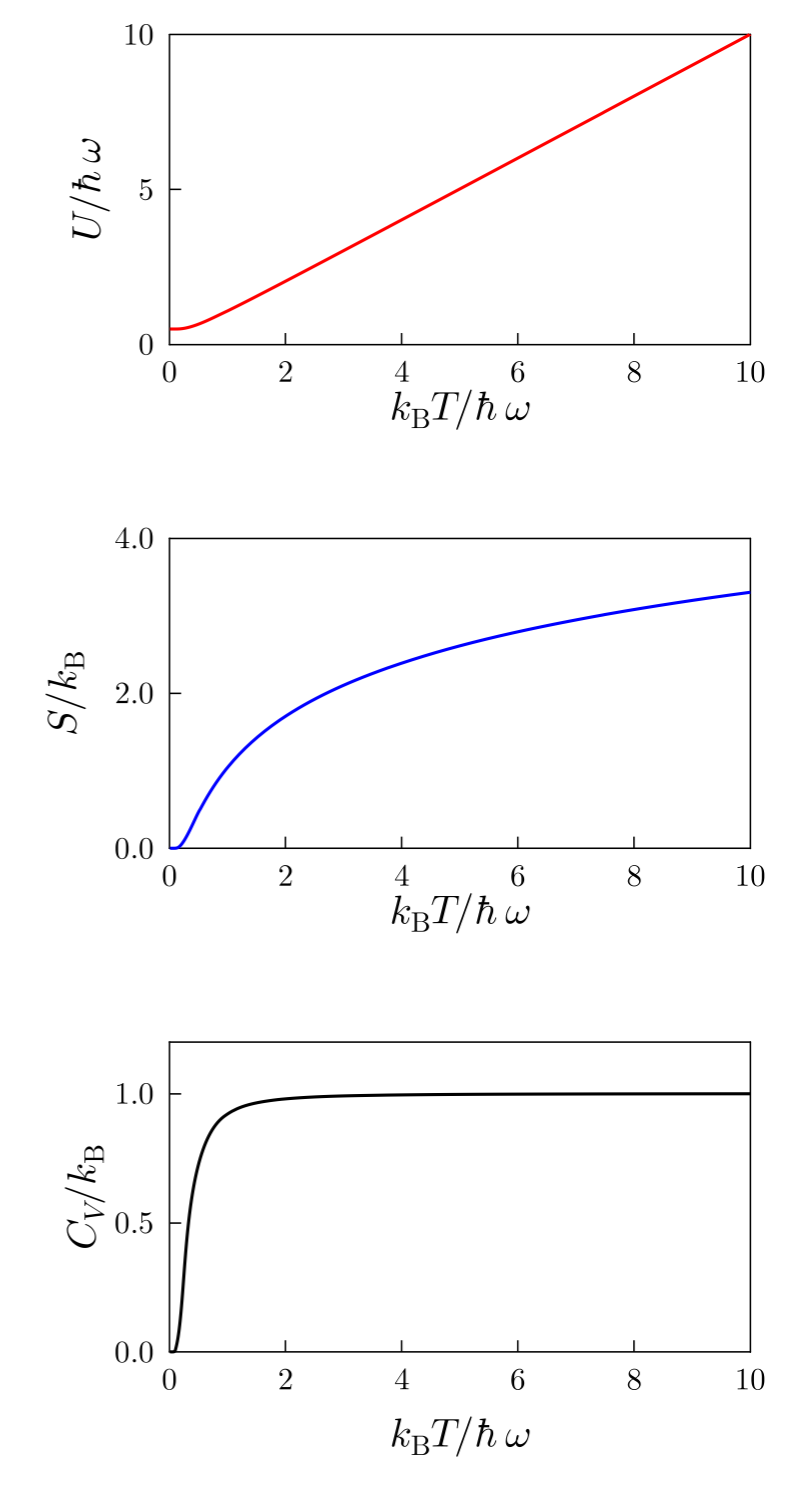
Plots of the normalized internal energy $U$, entropy $S$, and heat capacity $C_V$ for a quantum harmonic oscillator as a function of normalized temperature $k_B T / \hbar\omega$. These quantities are all derivable from the partition function $Z$ that we just calculated. For example, the heat capacity $C_V$ (bottom panel) correctly goes to zero at low temperatures, a key quantum effect, and approaches the classical value of $k_B$ at high temperatures.

The calculation we just performed is a classic one. The following video offers a very clear walkthrough of the derivation of the partition function and its consequences, which will be the subject of our next lesson. Although it starts from a classical perspective, the mathematical steps are identical.

Statistical Mechanics Lecture 4

This Stanford lecture by Leonard Susskind provides a masterful derivation of the Boltzmann distribution and the partition function.

First, watch the segment that defines the partition function Z as the normalization constant, arising from the Lagrange multiplier method: defining Z. This reinforces its role. Then, to get a preview of where we are heading, watch how the average energy E is derived from Z: deriving E from Z. This famous "trick" of differentiating \ln Z is a technique we will use extensively.

Conclusion

In this lesson, we have formally defined the quantum partition functions as traces of the statistical operators we derived previously. This moves them beyond being mere normalization constants and establishes them as the central computational objects in equilibrium statistical mechanics.

Key Takeaways:

The canonical partition function is formally defined as the trace of the Boltzmann operator: $Z = Tr (e^{- β H^})$ .
The grand partition function is defined similarly as a trace over the Fock space: $Ξ = Tr (e^{- β (H^- μ N^)})$ .
Evaluating the trace in the energy eigenbasis recovers the familiar sum-over-states expressions: $Z = \sum_{k} e^{- β E_{k}}$ .
We calculated the partition function for a quantum harmonic oscillator, a foundational model system, yielding $Z = [2 sinh (β ℏ ω /2)]^{- 1}$ .

Now that we have established what the partition function is and how to calculate it, the next logical step is to see how to use it. In our upcoming lesson, we will demonstrate that the partition function acts as a "generating function" for thermodynamics. We will derive expressions for key observables—internal energy, entropy, pressure, and particle number—by taking partial derivatives of the logarithm of the appropriate partition function, thus completing the bridge from microscopic quantum mechanics to macroscopic thermodynamics.

Recommended resources

1. The Partition Function as a Trace

2. The Grand Canonical Partition Function

3. Example: Partition Function of a Quantum Harmonic Oscillator

Conclusion