Instrumental Variables for Causal Inference in Fashion Research

The Problem of Endogeneity in the Photoshoot

Imagine you want to determine which lingerie outfit causally increases a "sexiness" rating in a boudoir photoshoot. You have data on various outfits and their corresponding sexiness scores. A simple Ordinary Least Squares (OLS) regression of Sexiness on Outfit would be:

The problem, as you know from your background in causal analysis, is endogeneity. A crucial unobserved variable here is the model's intrinsic Confidence. A more confident model might be more likely to choose a daring outfit and naturally project more sexiness, regardless of what she's wearing. This creates a confounding pathway.

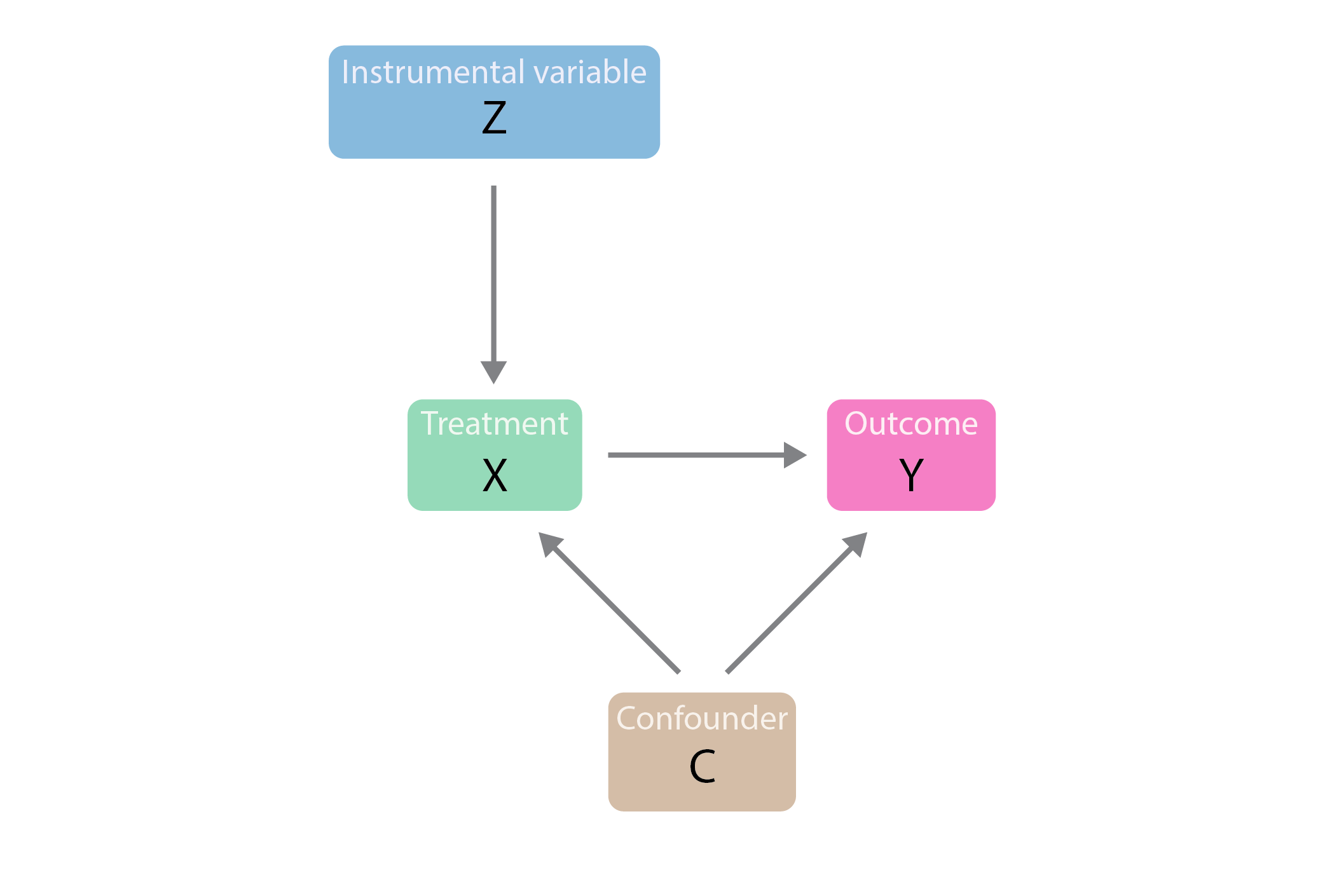
Because Outfit Choice (X) is correlated with Confidence (C), and Confidence also affects Perceived Sexiness (Y), the Outfit Choice variable is endogenous. The error term ${\eta }_i$ in our simple regression contains the effect of confidence, and it is correlated with our variable of interest, Outfit. Consequently, the OLS estimate for ${\beta }_1$ will be biased, likely overestimating the outfit's true effect by conflating it with the model's confidence.

To get a clearer intuition for this problem of endogeneity, let's watch a segment from an MIT OpenCourseWare lecture.

The Solution: Finding an Instrument

To isolate the true causal effect of the outfit, we need a source of variation in Outfit Choice that is exogenous—that is, uncorrelated with the unobserved Confidence. This is the role of an Instrumental Variable (IV).

A valid instrument, Z, must satisfy three core conditions, often referred to as relevance, exclusion, and independence.

Let's apply these conditions to our photoshoot scenario:

1. Relevance (Inclusion Restriction): The instrument Z must have a causal effect on the Outfit Choice (X). It has to actually make a difference in what outfit is chosen. This is testable and is known as the first stage.
2. Independence (or Exogeneity): The instrument Z must be as-if randomly assigned. It cannot be correlated with any unobserved factors that also affect Perceived Sexiness (Y), most notably our confounder, Confidence (C).
3. Exclusion Restriction: The instrument Z can only affect the Perceived Sexiness (Y) through its effect on Outfit Choice (X). There can be no direct causal path from Z to Y.

Finding a variable that satisfies these stringent conditions requires creativity and a deep understanding of the context—what econometricians call "institutional details." So, what could serve as an instrument for Outfit Choice?

Let’s consider a "wardrobe malfunction" or an "availability shock."

• Scenario: For a given shoot, the primary, high-impact lingerie set planned for use is suddenly discovered to be unusable (e.g., a clasp is broken, a key accessory is missing). This is an unexpected, random shock.
• Our Proposed Instrument (Z): A binary variable, malfunction, which equals 1 if the primary intended outfit is unavailable and 0 otherwise.

Now, let's rigorously evaluate this proposed instrument against the core assumptions using a helpful guide.

Based on that reading, how does our malfunction instrument hold up?

• Relevance: It's highly plausible that a malfunction forces a change of plans, causing a different, backup outfit to be used. malfunction will be correlated with Outfit Choice. We can test this.
• Independence: Is a random clasp breaking correlated with the model's baseline Confidence? Unlikely. This is the strength of using a random shock; it's "as-if" randomly assigned and plausibly independent of unobserved personal attributes.
• Exclusion Restriction: This is the most difficult assumption to defend. We must argue that the malfunction itself doesn't affect the final sexiness rating, other than by changing the outfit. For example, a critic could argue the malfunction soured the model's mood, which directly reduced her perceived sexiness. To defend the instrument, we would need to argue (and perhaps show with data, via a "falsification test") that such mood effects are negligible or non-existent. A good IV often feels "weird" because its connection to the outcome is not obvious, as explained in the "Causal Inference Mixtape" resource. The fact that a different outfit broke should, logically, have no bearing on the sexiness of the one that was ultimately worn and photographed.

How IV Estimation Works: The Two-Stage Intuition

With a valid instrument, we can estimate the causal effect using a method called Two-Stage Least Squares (2SLS).

1. First Stage: We isolate the portion of Outfit Choice that is exogenously driven by our instrument. We regress the endogenous variable on the instrument:

   $${\text{Outfit}}_i={\pi }_0+{\pi }_1\cdot {\text{malfunction}}_i+{\text{controls}}_i+v_i$$

   We then calculate the predicted values, ${\widehat{\text{Outfit}}}_i$. This predicted value represents the variation in outfit choice that is "clean"—free from the influence of the model's confidence.

2. Second Stage: We use these "clean" predicted values to estimate the effect on our outcome:

   $${\text{Sexiness}}_i={\beta }_0+{\beta }_{IV}\cdot {\widehat{\text{Outfit}}}_i+{\text{controls}}_i+{ϵ}_i$$

   Because ${\widehat{\text{Outfit}}}_i$ is now uncorrelated with the error term ${ϵ}_i$ (which still contains Confidence), our estimate for ${\beta }_{IV}$ is an unbiased estimate of the causal effect.

For a simple binary instrument like ours, this process simplifies to the intuitive Wald estimator:

The numerator is the "reduced form" effect—the total effect of the malfunction on sexiness. The denominator is the "first stage"—the effect of the malfunction on outfit choice. The ratio scales the overall effect to give us the per-unit causal effect of the outfit itself.

Let's return to the MIT lecture to see a formal derivation of this crucial result.

What are we Actually Estimating? The Local Average Treatment Effect (LATE)

A critical nuance, especially given your background, is that the IV estimate is not the Average Treatment Effect (ATE) for the entire population. It is the Local Average Treatment Effect (LATE). It is the average causal effect only for the sub-population whose behavior was changed by the instrument.

In the language of IV, we can partition our population into four groups:

• Compliers: Shoots where the malfunction caused a switch from the intended outfit to a backup. Their behavior "complied" with the instrument.
• Always-Takers: Shoots that would have used the backup outfit anyway, regardless of the malfunction.
• Never-Takers: Shoots that would have used the intended outfit anyway (perhaps by fixing it on the spot), regardless of the malfunction.
• Defiers: Shoots that would use the backup outfit if the primary is fine, but insist on the primary if it malfunctions. This group is usually assumed to not exist (the monotonicity assumption).

The IV estimate ${\beta }_{IV}$ gives us the causal effect of the outfit only for the compliers. The instrument provides no information about the effect for always-takers or never-takers. This locality is a fundamental aspect of the interpretation of IV results.

To deepen your understanding of this concept, we'll consult a foundational text in modern econometrics.

Conclusion

In this lesson, we have moved from prediction to the challenging world of causal inference. We designed a complete instrumental variable strategy to solve a practical problem: measuring the causal impact of an outfit on perceived sexiness while accounting for the powerful confounder of model confidence.

Key Takeaways:

• Endogeneity Bias: When an explanatory variable (like Outfit Choice) is correlated with the error term (due to an unobserved confounder like Confidence), OLS yields a biased estimate of the causal effect.
• Instrumental Variable (IV): An IV is an exogenous variable (Z) that influences the endogenous variable (X) but does not directly affect the outcome (Y), allowing us to isolate a "clean" source of variation.
• Three Core Conditions: A valid instrument must be relevant, satisfy the exclusion restriction, and be independent of the confounders. Designing a strategy involves creatively finding a plausible instrument and defending these assumptions.
• LATE Interpretation: The IV estimate is a Local Average Treatment Effect (LATE), representing the average causal effect specifically for the "compliers"—the group whose behavior was altered by the instrument.

This powerful technique allows you to move beyond correlation and uncover causal mechanisms, a cornerstone of rigorous analysis in both social research and efficiency optimization.

In our next lesson, we will explore the Generalized Method of Moments (GMM). GMM is a broader estimation framework that encompasses both OLS and IV as special cases, providing a unifying structure for many econometric models.