Adaptive Agent Modeling: Hotwife & Bull Dynamics

From Process Flows to Agent Behaviors

While DES answers questions about throughput and queues by modeling passive entities flowing through a fixed process, ABM addresses a different class of problems. It is designed for systems where the components are active, autonomous, and adaptive.

The core idea of ABM is to explicitly program the actions and interactions of these autonomous agents. Often, the rules governing each agent are quite simple, but when many agents interact, the collective result can be highly complex and unpredictable. This phenomenon is known as emergence.

The following short video from Complexity Explorer provides an excellent visual introduction to this concept using the classic example of fish schooling.

The Core Concepts of Agent-Based Modeling

To build an ABM, we must define the agents, their environment, and the rules that govern their behavior. Let's formalize these ideas.

A paper by Jackson et al., written as a guide for social psychologists, offers a clear definition of ABM and its central concepts. Given your background in social research, the perspective and examples in this text should resonate.

The key distinction between our previous lesson and this one is the shift in focus:

• In DES, the intelligence is in the process. Entities are passive.
• In ABM, the intelligence is in the agents. The process is emergent.

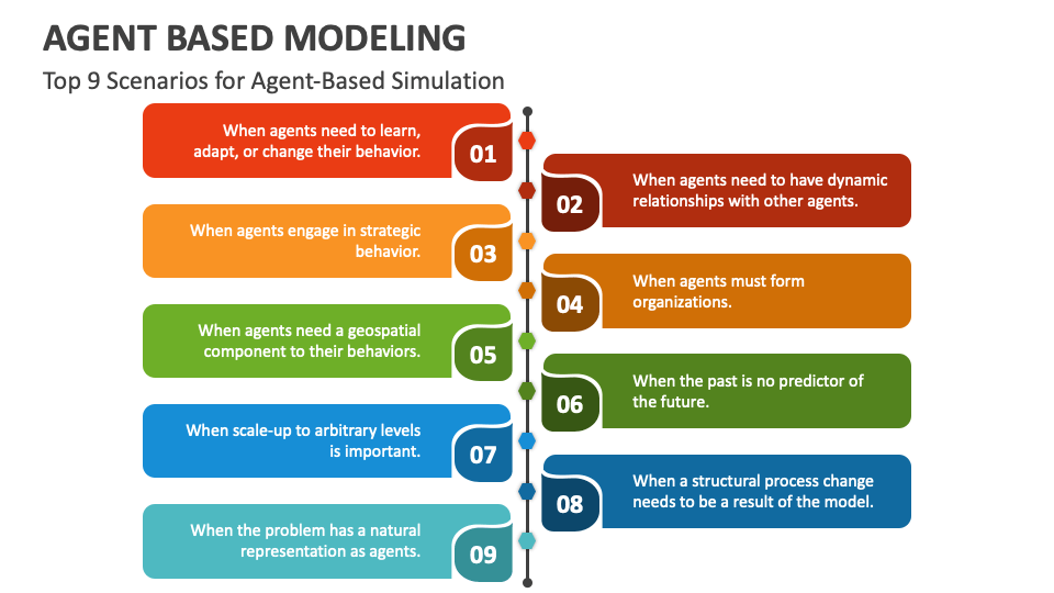
The infographic below highlights scenarios where ABM is the most appropriate simulation technique. Notice how many of these points—agents learning and adapting, dynamic relationships, and emergent structural change—are directly relevant to modeling the evolving intimacy dynamics between the hotwife and bull.

Constructing the Hotwife-Bull ABM: A Step-by-Step Guide

To construct our model, we need to define its fundamental components. The presentation slides from the University of Mannheim provide a concise checklist.

Now, let's apply this framework to our scenario. We will follow the 7-step guide proposed in the Jackson et al. paper to structure our model construction.

Here is how we can apply those seven steps to construct our model:

1. What are your world's dimensions?
The "world" is not a physical space. It's a temporal and state-based environment. The key dimensions are Time (advancing in discrete steps, e.g., days) and the State Space of each agent (their satisfaction, desire, etc.).

2. How do agents meet?
Agents don't meet spatially. They "interact" through a proposal-acceptance mechanism.

• The Hotwife agent initiates contact by proposing an encounter.
• This proposal is not random; it is triggered by her internal state (e.g., her Desire level crossing a certain threshold).

3. How do agents behave? (The Rules)
This is the core of the model. We define simple, if-then rules.

• Hotwife Agent:
  • State Variables: Satisfaction (scale 0-100), Desire (scale 0-100), Availability (a schedule).
  • Rule 1 (Desire Dynamics): At each time step, Desire decreases by a small amount (decay).
  • Rule 2 (Proposal): If Desire > 70 AND she is Available, propose an encounter to the Bull.
  • Rule 3 (Post-Encounter Update): If an encounter occurs, Satisfaction increases by a value dependent on the encounter type, and Desire resets to a low value (e.g., 10).
• Bull Agent:
  • State Variables: Availability (a schedule).
  • Rule 1 (Acceptance): If a proposal is received AND he is Available, accept the proposal with probability P_accept.

4. What is the payoff?
The primary "payoff" we are measuring is the Hotwife's Satisfaction level. This is the dependent variable that changes based on the interactions. This links back directly to the utility functions you modeled in the first module of the course.

5. How do agents change? (Adaptation)
This is where the model becomes dynamic and "intelligent." The agents' rules or states adapt based on experience.

• Example Adaptive Rule 1 (Learning from Rejection): Let's add a Confidence state to the Hotwife. If the Bull rejects a proposal, her Confidence decreases slightly. Her proposal rule can be modified to: If Desire > 70 AND Confidence > 50..., she becomes less likely to propose if repeatedly rejected.
• Example Adaptive Rule 2 (Learning Preferences): The Hotwife can maintain a memory of which encounter types yield the highest Satisfaction boost. She can adapt her proposal rule to be more likely to suggest activities that have been successful in the past.

6. How long does your world last?
We would run the simulation for a fixed duration, for example, 365 time steps (days), to observe how the dynamics unfold over a year. Since the model includes randomness (stochasticity), we would run it many times to get a distribution of outcomes.

7. What do you want to learn from your world?
This is the experimental phase. We define independent and dependent variables.

• Independent Variables (Parameters):
  • Bull's acceptance probability (P_accept).
  • Hotwife's desire decay rate.
  • Satisfaction values for different encounter types.
• Dependent Variables (Outputs to Measure):
  • The average Satisfaction level of the hotwife over the simulation run.
  • The frequency and timing of encounters (e.g., average time between encounters).
  • The emergent schedule: Do encounters cluster together, or are they spaced out?

By varying the parameters, we can run experiments to answer questions like: "How does a decrease in the bull's availability affect the hotwife's long-term satisfaction?" or "What is the optimal desire decay rate to maintain a high-satisfaction, stable pattern of encounters?"

A Concrete Example of a Social ABM

To see a fully realized social ABM in action, the following video describes the "DITCH" model, which simulates partner selection in diverse communities. This is a perfect analogue for our task. The researchers define agents with attributes and preferences, place them in a social network, and define rules for interaction (dating, partnership) to study emergent patterns of interethnic marriage.

Conclusion

This lesson concludes our exploration of simulation and our entire course on advanced operations research applications. We have journeyed from the precise logic of decision theory and game theory, through the probabilistic world of stochastic processes, to the powerful "what-if" engines of simulation.

Key Takeaways from this Lesson:

• Agent-Based Modeling (ABM) is a "bottom-up" simulation method that models a system as a collection of autonomous, interacting agents.
• The core of ABM is defining the agents, their environment, and the rules that govern their behavior and adaptation.
• Emergence is the key phenomenon studied with ABM, where complex, system-level patterns arise from simple, local interactions.
• To construct an ABM, you must clearly define the agents' states, their behavioral rules (often if-then logic), their mechanisms for interaction, and how they adapt over time.

You have now surveyed a vast and powerful toolkit for modeling, optimizing, and understanding complex systems. You have seen how deterministic optimization (like the Hungarian Method), strategic analysis (Game Theory), stochastic modeling (Markov Chains), and now simulation (DES and ABM) each provide a unique lens for analyzing problems—whether in the context of a boudoir photoshoot or the intricate dynamics of a non-monogamous relationship. The true power lies not just in mastering each tool individually, but in knowing which tool to apply to which problem, and how they can be combined—for instance, by using econometric methods to estimate the parameters that drive the rules in an agent-based model. I hope this journey has equipped you with new ways of thinking and a robust framework for your work as an optimizer and researcher.