Hierarchical Bayesian Models for Outfit-Pose Effectiveness

1. The Challenge of Grouped Data: Three Modeling Strategies

When faced with data organized into groups (in our case, test shoots), there are three common analytical strategies. Each represents a different assumption about the relationship between the groups. Let's consider these options in the context of estimating the "sexiness" score, $\theta$, of a specific outfit-pose combination.

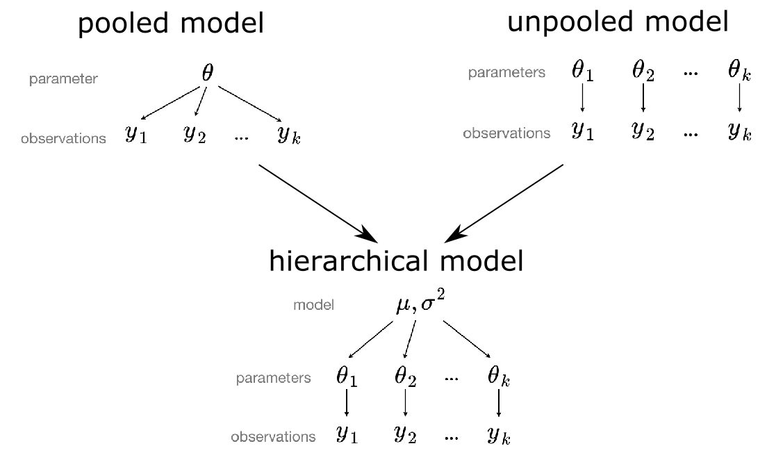
1. Complete Pooling: This approach assumes that the effectiveness of the outfit-pose is identical across all shoots. You would lump all the data together and estimate a single parameter, $\theta$, for the combo's effectiveness. This model is simple and uses all available data, leading to a low-variance estimate. However, it is likely biased, as it completely ignores any real differences between the shoots.

2. No Pooling: This strategy assumes that each shoot is entirely independent. You would fit a separate model for each shoot, estimating a distinct parameter ${\theta }_j$ for the combo's effectiveness in shoot $j$. This approach is unbiased and captures the unique characteristics of each shoot. However, for shoots with very few data points, the estimates will be highly uncertain and prone to overfitting. An unusually high or low rating from a single observation could drastically skew the result.

3. Partial Pooling (The Hierarchical Approach): This is the sophisticated middle ground. It assumes that while each shoot has its own effectiveness parameter ${\theta }_j$, these parameters themselves are related. Specifically, we model them as being drawn from a common, higher-level distribution. This allows the shoots to "borrow statistical strength" from one another. Estimates for data-poor shoots are regularized, or "shrunk," toward the overall average, preventing overfitting, while estimates for data-rich shoots are influenced more by their own data.

The diagram below illustrates these three structures. The pooled model has one parent parameter $\theta$ for all observations. The unpooled model has independent parameters ${\theta }_1,...,{\theta }_k$ for each group of observations. The hierarchical model introduces a higher-level model ($\mu ,{\sigma }^2$) that governs the group-level parameters ${\theta }_1,...,{\theta }_k$, creating a dependency between them.

Your background in statistics and econometrics has likely exposed you to the trade-offs between bias and variance. Hierarchical modeling offers a principled way to navigate this trade-off when dealing with grouped data.

2. A Conceptual Introduction to Hierarchical Modeling

To build a strong intuition for how hierarchical models work, we'll watch a presentation that walks through a classic case study: estimating radon levels across different counties in Minnesota. The problem is directly analogous to ours: some counties have many measurements (data-rich groups), while others have very few (data-poor groups).

The video beautifully illustrates that the hierarchical model isn't just a statistical trick; it's a more realistic representation of the world. It acknowledges that groups are neither identical nor completely independent, but share some degree of similarity.

3. Formalizing the Hierarchical Model and Sequential Updating

Let's translate this into the formal language of a Bayesian model for our photoshoot scenario. Suppose we have $J$ test shoots. For a given outfit-pose combination, let $s_j$ be the average sexiness rating from $n_j$ observations in shoot $j$.

A hierarchical model for this would have multiple levels:

1. Data Level (Likelihood): For each shoot $j$, we model the observed mean score $s_j$ as being drawn from a distribution centered on that shoot's "true" effectiveness, ${\theta }_j$. Assuming the ratings are approximately normal:

   $$s_j\sim \text{Normal}({\theta }_j,{\sigma }_j^2/n_j)$$

   Here, ${\sigma }_j^2$ is the variance of individual ratings within shoot $j$.

2. Group Level: Instead of assigning independent priors to each ${\theta }_j$, we model them as originating from a common group-level distribution. This is the core of the hierarchy.

   $${\theta }_j\sim \text{Normal}(\mu ,{\tau }^2)$$

   Here, $\mu$ is the global average effectiveness of the outfit-pose across all shoots, and ${\tau }^2$ is the variance, representing how much effectiveness tends to vary from shoot to shoot.

3. Hyperpriors: We place priors on the group-level parameters $\mu$ and $\tau$. These are called "hyperpriors" because they are priors on parameters of other priors.

   $$\mu \sim \text{Normal}(M,S^2)$$ $$\tau \sim \text{Half-Cauchy}(0,\gamma )$$

   We can set $M$ and $S$ to reflect some baseline belief about sexiness scores. A Half-Cauchy distribution is a common, weakly informative choice for a variance parameter like $\tau$.

This structure directly implements the "pooling of feedback." The information from all shoots informs the posterior distributions of $\mu$ and $\tau$. These, in turn, inform the posterior for each individual ${\theta }_j$. If shoot $k$ has a small $n_k$, its posterior for ${\theta }_k$ will be strongly influenced by the global estimates of $\mu$ and $\tau$.

Sequential Updating: "Today's Posterior is Tomorrow's Prior"

This idea of pooling information is deeply connected to the Bayesian principle of sequential updating. As you gather more data, you update your beliefs. The paper "Sequential Bayesian updating for Big Data" provides a clear, formal explanation of this process.

In our hierarchical model, this principle operates at the hyperparameter level. Imagine you analyze the first test shoot. You get a posterior for ${\theta }_1$, but you also get updated posteriors for $\mu$ and $\tau$. When data from the second shoot arrives, your prior for its effectiveness, ${\theta }_2$, is not a generic, uninformed guess. It is $p({\theta }_2)=\int p({\theta }_2|\mu ,\tau )p(\mu ,\tau |{\text{data}}_1)d\mu d\tau$. You are using the posterior belief about the global parameters—informed by the first shoot—as the prior for the second. This is how information is coherently pooled from one shoot to the next.

4. Visualizing the Impact: Shrinkage in Practice

The practical effect of this partial pooling is often called shrinkage, because the individual group estimates for data-poor groups are "shrunk" from their noisy sample means toward the more stable global mean.

The article "How to Fit Hierarchical Bayesian Models in R with brms" provides excellent visualizations of this effect. While you don't need to worry about the specific R code, the concepts and graphs are highly illustrative.

This shrinkage is precisely the mechanism that gives us more reliable estimates. For a new outfit-pose combination tested only a few times in one shoot, a non-hierarchical model might give an absurdly high or low score based on random chance. A hierarchical model, in contrast, would rightly be skeptical and pull that estimate closer to what's typical for other outfits, resulting in a more plausible and useful prediction.

Conclusion

In this lesson, we have explored how to use hierarchical Bayesian models to pool information across different groups of data. This approach provides a robust and principled solution to a common problem in data analysis.

Key Takeaways:

• When data is grouped, you can choose between complete pooling (high bias), no pooling (high variance), or partial pooling.
• Hierarchical Bayesian models implement partial pooling by adding a higher-level probability distribution that governs the parameters of the individual groups.
• This structure allows groups to "borrow statistical strength," leading to more stable and reliable estimates, especially for groups with sparse data. This effect is known as shrinkage.
• The process of pooling information is an application of sequential Bayesian updating, where the posterior belief about hyperparameters from one set of data becomes the prior for the next.

You have now seen how to move beyond single-agent decision theory to handle more complex data structures. In our next lesson, we will make another significant shift, from the world of a single decision-maker to the world of strategic interaction. We will enter the domain of game theory and start by modeling the boudoir photoshoot not as an optimization problem, but as a signaling game between the model and the photographer.