Welcome back. In our last lesson, we explored how to make a single, optimal decision when facing an uncertain future by comparing the principles of Expected Utility and Minimax Regret. We established a framework of actions, states, and payoffs, but assumed the decision was made with only our prior beliefs.
Today, we will advance from static to dynamic decision-making. Life rarely requires us to make choices in a vacuum; we often have the opportunity to gather more information before committing to a course of action. This lesson addresses the learning outcome of constructing a dynamic decision tree with information-gathering nodes. We will apply this to the hotwife scenario, optimizing her sequence of encounter planning choices by first considering whether to gather information about her bull's mood. This process is formally known as Bayesian pre-posterior analysis.
1. The Initial Decision: Structuring an Encounter Under Uncertainty
Let's begin by framing the decision problem without any new information. The hotwife wants to plan her next encounter with her bull to maximize her satisfaction, but she is uncertain about his current mood.
-
Actions (Encounter Plans):
- A1: Structured Plan: A pre-arranged, thematic encounter (e.g., a specific fantasy roleplay).
- A2: Spontaneous Plan: An open-ended, unstructured meeting that allows for improvisation.
-
States of Nature (Bull's Mood):
- S1: Adventurous: He is feeling high-energy and receptive to novelty and structured fantasy.
- S2: Relaxed: He is in a comfort-seeking mood, preferring spontaneous connection over complex plans.
-
Payoffs (Hotwife's Satisfaction Utility):
Based on her preferences, we can construct a payoff matrix.
| Action | S1: Adventurous | S2: Relaxed |
|---|---|---|
| A1: Structured | 90 | 50 |
| A2: Spontaneous | 60 | 85 |
- Prior Probabilities, P'(S):
Based on past experience, she has a prior belief about his likely mood:- P'(S1: Adventurous) = 0.4
- P'(S2: Relaxed) = 0.6
This "prior analysis" branch of the decision tree involves calculating the expected utility for each action using these initial probabilities.
- EU(A1: Structured) = (90 × 0.4) + (50 × 0.6) = 36 + 30 = 66
- EU(A2: Spontaneous) = (60 × 0.4) + (85 × 0.6) = 24 + 51 = 75
Without any new information, the optimal decision is to choose the Spontaneous Plan (A2), yielding an expected utility of 75. This value is known as the Expected Value Under Uncertainty (EVUU). It is our baseline.
2. The Opportunity to Learn: Pre-Posterior Analysis
What if the hotwife could reduce her uncertainty before choosing a plan? She could perform an "experiment" to get a signal about the bull's mood. This is the core of pre-posterior analysis: deciding whether it's worth gathering information before it is obtained.
The following paper provides the formal framework for this process. It details the variables and the sequence of calculations required.
Value of Bayesian Pre-Posterior Information for Enhancing Life ...
This paper formally describes the methodology of pre-posterior analysis, which is exactly what we are implementing. It shows how to structure the problem and calculate the value of new information.
First, read the introduction and Section 4 to understand the purpose of this method. Then, study Section 4.1, which defines the key components: alternatives (A), states of nature (S), experiments (e), results (r), prior probabilities P'(S), and conditional probabilities P(r|S, e). Finally, examine the decision tree in Figure 4 and the summary of methodological steps in Figure 5 to visualize the entire process.
Let's apply this framework to our scenario:
- Experiment (e): Send a suggestive, open-ended text message. Let's assume a small utility cost of
2for this action, representing the effort and potential for misinterpretation. - Outcomes/Results (r): His reply serves as a signal.
- r1: Enthusiastic Reply: A witty, high-energy response.
- r2: Warm Reply: A simple, affectionate response.
- Conditional Probabilities, P(r|S, e): This is the reliability of the signal. We need to estimate the probability of getting each type of reply, given his true mood.
- P(r1 | S1: Adventurous) = 0.8 (An adventurous mood is likely to produce an enthusiastic reply).
- P(r1 | S2: Relaxed) = 0.3 (A relaxed mood could still produce an enthusiastic reply, but it's less likely).
- From these, we can infer the complementary probabilities:
- P(r2 | S1: Adventurous) = 1 - 0.8 = 0.2
- P(r2 | S2: Relaxed) = 1 - 0.3 = 0.7
3. Updating Beliefs: From Priors to Posteriors
Given the signal's reliability, we can now use Bayes' theorem to calculate the posterior probabilities, P''(S|r, e). This answers the question: "After seeing his reply, what is the new probability of him being in an adventurous vs. relaxed mood?"
First, we need the marginal probability of each reply, P(r|e):
- P(r1) = P'(S1)P(r1|S1) + P'(S2)P(r1|S2) = (0.4)(0.8) + (0.6)(0.3) = 0.32 + 0.18 = 0.50
- P(r2) = P'(S1)P(r2|S1) + P'(S2)P(r2|S2) = (0.4)(0.2) + (0.6)(0.7) = 0.08 + 0.42 = 0.50
Now we apply Bayes' theorem to find the posterior probabilities:
If she receives an Enthusiastic Reply (r1):
- P''(S1 | r1) = (0.8 × 0.4) / 0.50 = 0.32 / 0.50 = 0.64
- P''(S2 | r1) = (0.3 × 0.6) / 0.50 = 0.18 / 0.50 = 0.36
The enthusiastic reply significantly increases her belief that he is in an adventurous mood (from 40% to 64%).
If she receives a Warm Reply (r2):
- P''(S1 | r2) = (0.2 × 0.4) / 0.50 = 0.08 / 0.50 = 0.16
- P''(S2 | r2) = (0.7 × 0.6) / 0.50 = 0.42 / 0.50 = 0.84
The warm reply strongly suggests he is in a relaxed mood, updating her belief from 60% to 84%.
4. Solving the Dynamic Decision Tree
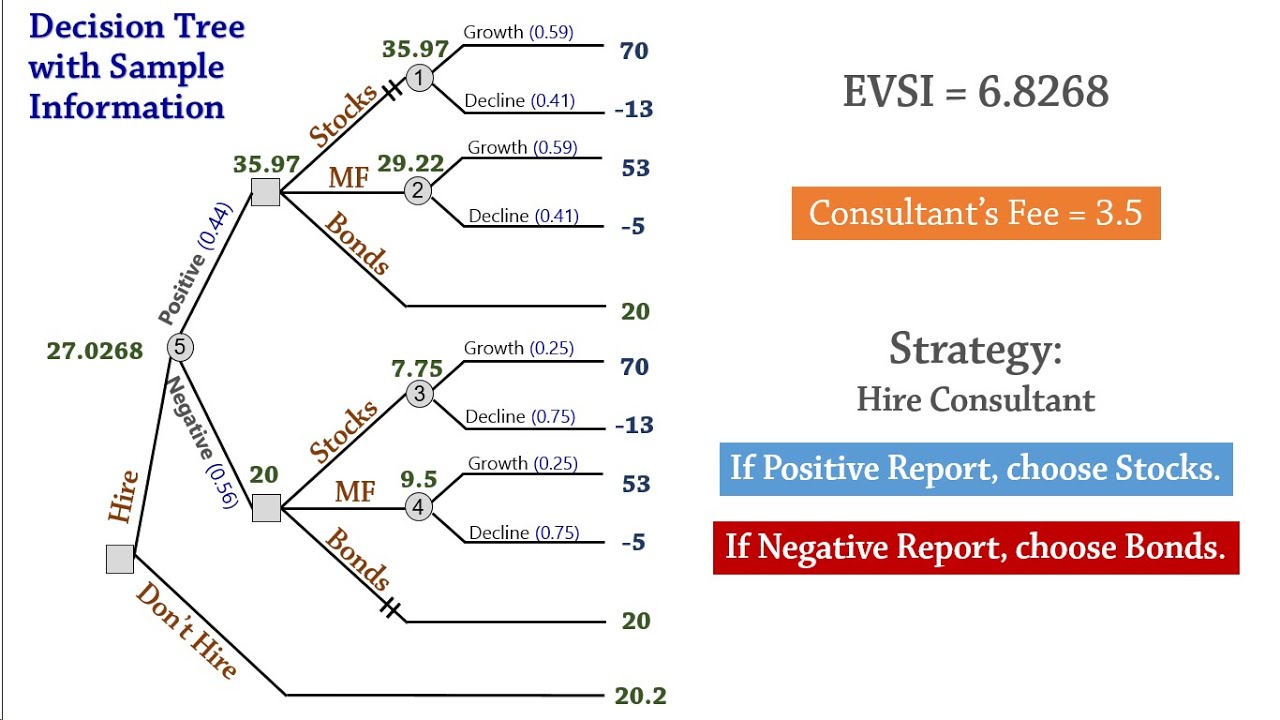
We can now construct and solve the full tree using the "rollback" method, moving from right to left. The tree has two main branches at the root: "Send Text" and "Don't Send Text".
Branch 1: Don't Send Text (Prior Analysis)
We already solved this. The value of this branch is the EVUU, which is 75.
Branch 2: Send Text (Posterior Analysis)
This branch begins with a chance node representing the bull's reply.
-
Path 1: Enthusiastic Reply (r1) occurs (Prob = 0.50)
We make a decision using the posterior probabilities P''(S|r1):- EU(A1: Structured | r1) = (90 × 0.64) + (50 × 0.36) = 57.6 + 18 = 75.6
- EU(A2: Spontaneous | r1) = (60 × 0.64) + (85 × 0.36) = 38.4 + 30.6 = 69
- Optimal action after r1 is Structured (A1), with an expected utility of 75.6.
-
Path 2: Warm Reply (r2) occurs (Prob = 0.50)
We make a decision using the posterior probabilities P''(S|r2):- EU(A1: Structured | r2) = (90 × 0.16) + (50 × 0.84) = 14.4 + 42 = 56.4
- EU(A2: Spontaneous | r2) = (60 × 0.16) + (85 × 0.84) = 9.6 + 71.4 = 81
- Optimal action after r2 is Spontaneous (A2), with an expected utility of 81.
Now, we roll back to the "Send Text" node. The expected value of this branch is the weighted average of the outcomes, before knowing the reply. This is the Expected Value with Sample Information (EVwithSI).
- EVwithSI = [P(r1) × EU(Optimal Action|r1)] + [P(r2) × EU(Optimal Action|r2)]
- EVwithSI = (0.50 × 75.6) + (0.50 × 81) = 37.8 + 40.5 = 78.3
5. Making the Final Decision and Valuing Information
We have the expected utility of both initial choices.
- Don't Send Text: Expected Utility = 75
- Send Text: Gross Expected Utility = 78.3
The Expected Value of Sample Information (EVSI) is the increase in expected utility gained from the information.
- EVSI = EVwithSI - EVUU = 78.3 - 75 = 3.3
This means the information from the text message is worth 3.3 utility points, on average. Now we compare the final net values of the two main branches:
- Value(Don't Send Text) = 75
- Value(Send Text) = EVwithSI - Cost(Experiment) = 78.3 - 2 = 76.3
Since 76.3 > 75, the optimal strategy is to Send the Text.
The complete, optimal policy is:
- Send the text message to gather information about his mood.
- If the reply is enthusiastic, choose the Structured Plan.
- If the reply is warm, choose the Spontaneous Plan.
For a deeper dive into calculating the value of information, including the concept of the Expected Value of Perfect Information (EVPI) which provides an upper bound on what you should pay for any information, the following document is a useful reference.
[PDF] Value of Information in Decision Trees
This document provides several methods for calculating the value of information, distinguishing between perfect information (EVPI) and imperfect or sample information (which we calculated as EVSI).
Skim the section on the Expected Value of Perfect Information to understand it as the theoretical maximum value of information. Then, review the DriveTek problem, which illustrates a more complex scenario with imperfect information, similar in structure to our problem.
Conclusion
In this lesson, you have moved beyond static decisions to construct a dynamic decision tree that incorporates an information-gathering step. By applying Bayesian pre-posterior analysis, you were able to quantify the value of a signal and formulate an adaptive strategy that changes based on new evidence.
Key Takeaways:
- Dynamic Decision Trees model sequential choices, where initial decisions can be about whether to acquire information.
- Pre-posterior analysis is the formal method for evaluating the worth of an "experiment" before it's conducted.
- Bayes' Theorem is the engine that updates your prior beliefs into posterior beliefs based on the information received.
- The Expected Value of Sample Information (EVSI) measures the gross increase in expected utility from imperfect information, which must be weighed against the cost of obtaining it.
- The final output is not just a single choice, but a contingent policy that dictates the best action for each possible outcome of the information-gathering step.
In our next lesson, we will transition from decision theory to game theory. The signal in today's lesson—the text message—will be formalized as we "Model the photographer-model interaction as a signaling game." We will explore how actions can be interpreted as signals that convey private information between strategic agents.