Calculating Spot and Forward Rates from Bond Prices

Introduction

In our last lesson, we developed a conceptual understanding of the term structure of interest rates, learning to interpret the economic signals sent by different shapes of the yield curve. We are now ready to transition from this qualitative overview to the quantitative mechanics that underpin it.

This lesson focuses on calculating the fundamental components of the yield curve: spot rates and forward rates. Unlike the yield-to-maturity (YTM) of a coupon bond, which is an average rate over the bond's life, spot and forward rates are the "pure" interest rates for specific time horizons. Mastering their calculation is crucial for accurately pricing any financial instrument with future cash flows. We will use a powerful technique called bootstrapping to extract these rates directly from the prices of bonds traded in the market.

Spot Rates: The Pure Cost of Money Over Time

A spot rate, denoted as $s_{t}$ , is the annualised rate of return on a zero-coupon bond that matures at time $t$ . Since a zero-coupon bond has only one cash flow—its principal at maturity—its yield is not an average of different rates over time. It represents the pure, risk-free interest rate for a single, specific term.

Any coupon-paying bond can be deconstructed into a series of zero-coupon payments: each coupon is a small zero-coupon bond, and the final principal is a large one. Therefore, the correct way to price a coupon bond is to discount each of its cash flows at the specific spot rate corresponding to the timing of that cash flow.

The price ( $P$ ) of an $n$ -year bond with annual coupons ( $C$ ) and face value ( $F$ ) is given by:

P = \frac{C}{( 1 + s _{1} ) ^{1}} + \frac{C}{( 1 + s _{2} ) ^{2}} + \dots + \frac{C + F}{( 1 + s _{n} ) ^{n}}

Notice how each cash flow is discounted by a different spot rate, $s_{t}$ , that matches its maturity $t$ .

To see this principle in action, let's review a formal definition and an example of pricing a bond using a given set of spot rates.

The Term Structure of Interest Rates, Spot Rates, and Yield ...

This document from the University of Pennsylvania's Wharton School provides a precise introduction to spot rates and their application.

First, read the initial section on spot rates. This part defines spot rates using one- and two-year zero-coupon bonds. Next, study EXAMPLE 5A.1. Pay close attention to how the bond's price is calculated in Equation A.1. This equation demonstrates how a 2-year coupon bond is valued by discounting its year 1 and year 2 cash flows using two different spot rates, r_1 and r_2.

Deriving Spot Rates: The Bootstrapping Method

In practice, the market does not offer a complete set of zero-coupon government bonds for every maturity. What we usually have is a par curve, which consists of the yields for coupon-bearing bonds that are trading at their par value (i.e., price = face value). When a bond trades at par, its coupon rate equals its yield-to-maturity (YTM).

Our task is to extract the pure spot rate curve from this par curve. The method we use is called bootstrapping. It's an iterative process where we "pull ourselves up by our own bootstraps" by using the spot rate(s) we just calculated to solve for the next one in the sequence.

The following video provides an excellent, step-by-step demonstration of this process.

Bootstrapping Spot Rates From the Par Curve

This video from Ryan O'Connell, CFA, FRM, clearly explains how to bootstrap spot rates from a par curve, first with a pen-and-pad calculation and then in Excel.

Please watch the first six minutes, which cover the core logic and calculations: Introduction: The video introduces the par curve and sets up the problem. The key insight is that for a one-year bond with a single cash flow, the 1-year spot rate is equal to the 1-year par rate. This gives us our starting point. Calculating the 2-Year Spot Rate: Follow this calculation closely. We know the price of the 2-year par bond (it's $100), the coupon rate (from the par curve), and the 1-year spot rate we just found. We can write the pricing equation with only one unknown: the 2-year spot rate, s_2. By rearranging the formula, we solve for s_2. Calculating the 3-Year Spot Rate: The process repeats. Using the now-known s_1 and s_2, we discount the first two cash flows of the 3-year par bond. The only remaining unknown is s_3, which we solve for.

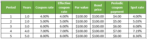
The logic of bootstrapping can be summarized as follows:

Step 1 (t=1): A 1-year par bond has one payment at maturity. Its price is $100 = \frac{100 + C _{1}}{1 + s _{1}}$ , where $C_{1}$ is the 1-year par coupon rate. Since for a par bond $C_{1} = Y T M_{1}$ , this simplifies to $s_{1} = Y T M_{1}$ .
Step 2 (t=2): A 2-year par bond has a price of $100. We know its coupon $C_{2}$ and the spot rate $s_{1}$ . We solve for $s_{2}$ in the equation: $100 = \frac{C _{2}}{( 1 + s _{1} ) ^{1}} + \frac{100 + C _{2}}{( 1 + s _{2} ) ^{2}}$
Step n: For an $n$ -year par bond, we know $s_{1}, s_{2}, ..., s_{n - 1}$ from previous steps. We solve for $s_{n}$ : $100 = t = 1 \sum n - 1 \frac{C _{n}}{( 1 + s _{t} ) ^{t}} + \frac{100 + C _{n}}{( 1 + s _{n} ) ^{n}}$

The table below shows a typical result of this process, where spot rates are derived from a series of bonds with different coupon rates.

This table shows a set of par bonds with increasing maturities and coupon rates. The rightmost column, "Spot rate," shows the result of the bootstrapping calculation for each year. Note that for Year 1, the spot rate equals the coupon rate, but for subsequent years, the spot rate diverges.

Forward Rates: Implied Future Interest Rates

Once we have the spot rate curve, we can derive another crucial set of rates: forward rates. A forward rate is an interest rate, agreed upon today, for a loan that will be made at some point in the future.

The key insight is based on the principle of no-arbitrage. An investor should be indifferent between two strategies:

Investing for two years at the 2-year spot rate ( $s_{2}$ ).
Investing for one year at the 1-year spot rate ( $s_{1}$ ) and simultaneously arranging to reinvest the proceeds for the second year at a locked-in rate.

This locked-in rate for the second year is the one-year forward rate, starting one year from now, denoted $f_{1, 2}$ (or simply $f_{1}$ when the period is one year).

The no-arbitrage condition means the future value from both strategies must be equal:

(1 + s_{2})^{2} = (1 + s_{1})^{1} \times (1 + f_{1, 2})^{1}

This relationship is perfectly illustrated in the following diagram.

This diagram shows two paths to get from \$1 today to a future value in two years. The bottom path uses the 2-year spot rate (6%). The top path uses the 1-year spot rate (5%) followed by the 1-year forward rate ("F"). By the no-arbitrage principle, the future values must be equal, allowing us to solve for F.

We can rearrange the formula to solve for the forward rate:

f_{1, 2} = \frac{( 1 + s _{2} ) ^{2}}{( 1 + s _{1} )} - 1

More generally, the one-year forward rate starting $n - 1$ years from now is given by:

f_{n - 1, n} = \frac{( 1 + s _{n} ) ^{n}}{( 1 + s _{n - 1} ) ^{n - 1}} - 1

The following video works through a full example, first bootstrapping the spot rates and then using those spot rates to calculate the implied forward rates.

CFA Level 2 | Fixed Income: Bootstrapping Spot Rates from Par Rates & No-Arbitrage Valuation

Fabian Moa, CFA, FRM provides another clear, numerical example covering both parts of our learning outcome.

First, watch the bootstrapping section from the beginning. This will reinforce the calculation process you saw in the previous video. Then, continue to the next section from calculating forward rates. This segment shows how to use the spot rates just derived (s_1, s_2, s_3) to compute the one-year forward rates starting one and two years from now (f_{1,2} and f_{2,3}).

Conclusion

In this lesson, we have moved from a conceptual view of the yield curve to its practical construction. We've defined the fundamental building blocks of the term structure and learned the quantitative methods to calculate them from market data.

Key Takeaways:

Spot rates ( $s_{t}$ ) are the pure, zero-coupon yields for specific maturities and are the theoretically correct rates for discounting single cash flows.
Bootstrapping is an iterative process used to derive the spot rate curve from the prices of coupon-bearing bonds (often a par curve).
Forward rates ( $f_{n - 1, n}$ ) are future interest rates implied by today's spot rate curve, determined by a no-arbitrage argument.
The relationship between spot and forward rates is captured by the formula: $(1 + s_{n})^{n} = (1 + s_{n - 1})^{n - 1} (1 + f_{n - 1, n})$ .

With these quantitative tools in hand, we are now equipped to revisit the theories of the term structure in our next lesson. We will explore how the Expectations Hypothesis and Liquidity Preference Theory provide formal explanations for the relationship between the spot and forward rates we've just learned to calculate.

Recommended resources

Introduction

Spot Rates: The Pure Cost of Money Over Time

Deriving Spot Rates: The Bootstrapping Method

Forward Rates: Implied Future Interest Rates

Conclusion