LTS Magnet Design and Field Limits

Introduction

In our last lesson, we established the fundamental physics of Type-II superconductors, defining the critical surface $J_c(B,T)$ that bounds their operational limits. We saw that a high upper critical field ($B_{c2}$) and a high critical current density ($J_c$) are prerequisites for building powerful magnets.

This lesson bridges the gap from that theoretical foundation to real-world engineering. We will focus on the workhorses of the high-field world: Low Temperature Superconductors (LTS). Our goal is to analyze LTS magnet designs using NbTi and Nb3Sn and calculate their field limits, directly addressing this lesson's learning outcome.

We will explore why these materials are not used as simple wires but as complex composites. Most importantly, we will introduce the "load-line" analysis—a graphical method that is the standard engineering tool for determining the maximum field a given magnet design can achieve. This is a core competency for anyone involved in magnet design, and it will be a recurring theme as we move forward.

1. The Two LTS Workhorses: Niobium-Titanium (Nb-Ti) and Niobium-Tin (Nb3Sn)

While many materials exhibit Type-II superconductivity, two alloys have dominated the field of LTS magnets for decades.

• Niobium-Titanium (Nb-Ti): This is a ductile alloy, making it relatively easy to manufacture into long, flexible wires. It has been the standard for MRI magnets, particle accelerator magnets (like the majority of the LHC), and research magnets for generating fields up to about 10 T.
• Niobium-Tin (Nb3Sn): This is an intermetallic compound with a specific crystal structure (A15). It is notoriously brittle but offers superior superconducting properties compared to Nb-Ti. It is the material of choice for pushing beyond the limits of Nb-Ti, enabling fields in the 10 T to ~23 T range.

The fundamental performance difference is clear from their critical field vs. temperature curves.

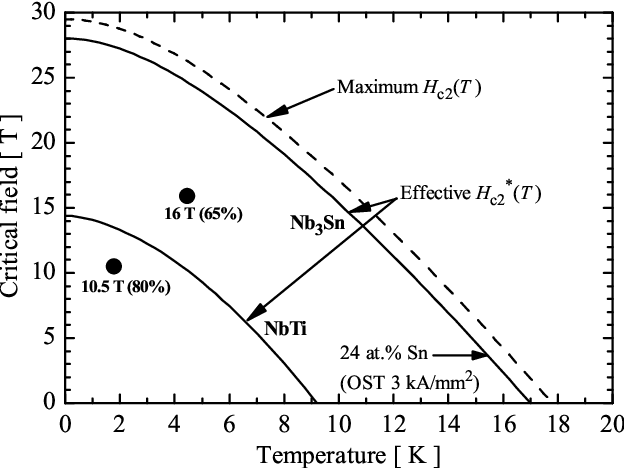
As the graph shows, Nb3Sn possesses a significantly higher critical temperature ($T_c\approx 18$ K vs. $\approx 9.2$ K) and upper critical field ($B_{c2}\approx 28$ T vs. $\approx 14.5$ T).

However, their mechanical properties introduce a crucial divergence in magnet construction:

• Nb-Ti: Being ductile, it can be manufactured into a final wire and then wound into a coil.
• Nb3Sn: Its brittleness means it cannot be significantly bent or strained after the Nb3Sn compound is formed. Therefore, magnets are built using a "wind-and-react" technique. The coil is wound using unreacted, ductile precursor wires (containing separate Nb and Sn components). The entire coil is then heat-treated for hundreds of hours at $\sim 650^{\circ }$C to form the brittle Nb3Sn compound in situ. This process adds significant complexity and introduces challenges related to thermal expansion and strain management, which are critical aspects of the magnet's mechanical design.

2. From a Superconductor to a Practical Wire

You might wonder why we don't simply use a solid block of Nb-Ti to wind a coil. A practical superconducting wire is a sophisticated composite, engineered for stability, protection, and performance. The reasons for this complexity are deeply tied to the physics we have discussed.

The following reading from a CERN report provides an excellent and comprehensive explanation of the design of practical superconducting strands and cables.

To summarize the key points from the reading:

• Fine Filaments ($\mu$m diameter):

  • Flux Jump Stability: Large superconducting regions are prone to magneto-thermal instabilities called "flux jumps," where a small thermal disturbance can cause a cascade that quenches the magnet. Smaller filaments are inherently more stable.
  • Reduced Magnetization: Persistent screening currents in the filaments create unwanted magnetization, which generates field errors (bad for accelerator optics) and AC losses during field ramps. The magnitude of this effect is proportional to the filament diameter, so smaller is better.

• Copper Matrix (Stabilizer):

  • Stabilization: Provides a low-resistance path for current to flow around a small, temporary "hot spot," allowing the filament to cool down and recover its superconducting state.
  • Quench Protection: In an irreversible quench, the superconductor becomes highly resistive. The copper matrix provides a safe, parallel path for the massive current to flow, preventing the energy from being dumped into a tiny volume, which would melt the wire.

• Twisting:

  • Filaments within a strand are twisted to prevent them from acting like a single large conductor in a changing magnetic field, which would create large eddy current loops and high AC losses.
  • Strands within a cable are also twisted for the same reason on a larger scale.

• Rutherford Cable: Multiple strands are flattened and twisted into a cable to carry very high currents (thousands of amps) in a compact, mechanically stable form that is convenient for winding.

3. Calculating the Field Limit: Load-Line Analysis

Now we arrive at the central task: how do we predict the maximum field a magnet will achieve? The method involves comparing the performance of the superconducting wire with the characteristics of the magnet coil it's wound into. This is done graphically using a load-line analysis.

Here's the breakdown of the concept:

1. The Critical Curve: For a fixed operating temperature (e.g., 4.2 K or 1.9 K), the critical surface $J_c(B,T)$ becomes a 2D line, $J_c(B)$. Multiplying by the superconductor area in a strand gives the critical current, $I_c(B)$. This curve represents the absolute performance limit of the wire. Any current/field combination above this line is impossible.

2. The Magnet Load Line: For any given magnet coil, the magnetic field it produces is directly proportional to the current flowing through it. This gives a linear relationship: $B=k\cdot I$, where $k$ is a constant that depends only on the coil's geometry. This straight line on the I-B plot is the magnet load line.

3. Peak Field vs. Bore Field: The field is not uniform across the coil winding. There is always a "hot spot" where the field is highest. This peak field on the conductor is what determines if the superconductor quenches, not the useful field in the magnet's bore. Therefore, we must use a load line for the peak field, $B_{peak}$. The ratio ${\lambda }_{peak}=B_{peak}/B_{bore}$ is a crucial design parameter determined from electromagnetic modeling.

4. The Short-Sample Limit: The intersection of the material's critical curve and the magnet's peak field load line defines the theoretical maximum current ($I_{ss}$) and bore field ($B_{ss}$) the magnet can reach. This is called the short-sample limit because the critical curve is measured on a short, straight sample of the wire before it's wound into the magnet.

5. Operating Margin: For safety and stability, magnets are never operated at 100% of their short-sample limit. A typical operating margin is 20%, meaning the operational current $I_{op}$ is set to be 80% of $I_{ss}$. This provides a buffer against small temperature fluctuations or mechanical disturbances that could trigger a quench.

The following reading explains this process with the relevant formulas for a dipole magnet.

4. Application: Case Study of an 11 T Dipole

Let's apply these concepts to a practical example. The CERN report contains a superb case study that walks through the preliminary design steps for an 11 T Nb3Sn dipole magnet, a field level that requires moving from Nb-Ti to Nb3Sn. This exercise will allow you to perform the core calculations yourself.

First, it is critical to distinguish between the different definitions of current density, as they link the physics of the superconductor to the engineering of the magnet.

• Superconductor Current Density ($j_{sc}$): The current density within the superconducting filaments themselves. This is the physically fundamental quantity related to the critical surface.
• Engineering Current Density ($j_e$): The current density averaged over the entire strand cross-section, including the copper matrix.
• Overall Current Density ($j_o$): The current density averaged over the entire coil cross-section, including insulation and voids. This is the quantity that directly generates the magnetic field in the bore.

The ratio between these is determined by the filling factor of the coil. The resource LINK provides a good overview of this in section "II.6.3.7.1 Filling factor and different current densities".

Conclusion

Key Takeaways:

• Nb-Ti (ductile, $\sim$10 T limit) and Nb3Sn (brittle, $\sim$23 T limit) are the primary LTS materials, each with distinct manufacturing requirements due to their mechanical properties.
• Practical superconducting wires are complex composites of micron-thin filaments in a copper matrix, which are twisted into strands and cabled to ensure thermal stability and quench protection.
• Load-line analysis is the fundamental engineering method for determining a magnet's performance limit. It involves finding the intersection of the superconductor's critical curve ($I_c(B)$) and the coil's load line ($B_{peak}\propto I$).
• Magnets are operated with a significant safety margin (e.g., at 80% of the short-sample limit) to ensure reliable operation.

Next Lesson Preview:
We have now covered the design and limits of both resistive and LTS continuous-field magnets. The next logical step is to explore the materials that promise to push beyond the ~23 T limit of Nb3Sn: High Temperature Superconductors (HTS). We will evaluate materials like REBCO, discuss their advantages (higher fields, larger temperature margins), and analyze the unique challenges they present for magnet construction.