Calculating Asset Correlation and Covariance

Hello! Welcome to the fourth lesson in our "Foundations" module.

In our previous lesson, we explored how individual asset returns can be modeled using probability distributions, focusing on the normal distribution for log returns and the resulting log-normal distribution for prices. We saw this is a powerful, but imperfect, model.

So far, we've only analyzed assets in isolation. However, markets are interconnected systems. The price of Ethereum doesn't move in a vacuum; it's influenced by and influences the price of Bitcoin and the broader crypto market. Understanding these inter-relationships is fundamental to building robust strategies, especially for diversification and relative value trading.

Today, we will learn how to quantify the relationship between two asset price series by calculating and interpreting covariance and correlation. This will allow us to move from analyzing single assets to understanding how they move together.

1. The Theory: Measuring Co-movement

At its core, we want to answer a simple question: when Asset X goes up, what does Asset Y tend to do?

Does it also go up? (Positive relationship)
Does it tend to go down? (Negative relationship)
Is there no discernible pattern? (No relationship)

Covariance and correlation are the two primary statistical tools we use to answer this.

To get a solid theoretical grounding, let's watch a few segments from a video by Prof. Steve Brunton, who provides excellent mathematical intuition.

Covariance and Correlation in Probability

This video, "Covariance and Correlation in Probability", lays out the theoretical groundwork. We'll focus on the core definitions and the intuition behind them.

Please watch the following segments: Introduction (00:00 - 03:55): Pay attention to the definition of covariance as the expected value of the product of deviations from the mean: \text{Cov}(X,Y) = \mathbb{E}[(X-\mu_X)(Y-\mu_Y)]. Note how this is a natural extension of the formula for variance. Visual Intuition (03:55 - 08:02): This part uses scatter plots to visually demonstrate what high positive, low positive, and zero covariance look like. This is key for developing an intuitive feel for the metric. Correlation as Normalized Covariance (15:45 - 18:20): This section introduces correlation and explains its most important property: it's a normalized measure that is invariant to scaling. This addresses the major shortcoming of covariance.

Distinguishing Covariance and Correlation

As the video explains, these two concepts are related but serve different purposes. Let's crystallize the differences.

Covariance measures only the direction of the linear relationship.
- Positive value: The two variables tend to move in the same direction.
- Negative value: They tend to move in opposite directions.
- Its magnitude is hard to interpret because it depends on the variance of the variables themselves. For example, the covariance between BTC/USD and ETH/USD will be much larger than the covariance between two low-priced altcoins, even if the degree of co-movement is the same.
Correlation measures both the direction and the strength of the linear relationship.
- It is the covariance normalized by the product of the standard deviations of the two variables.
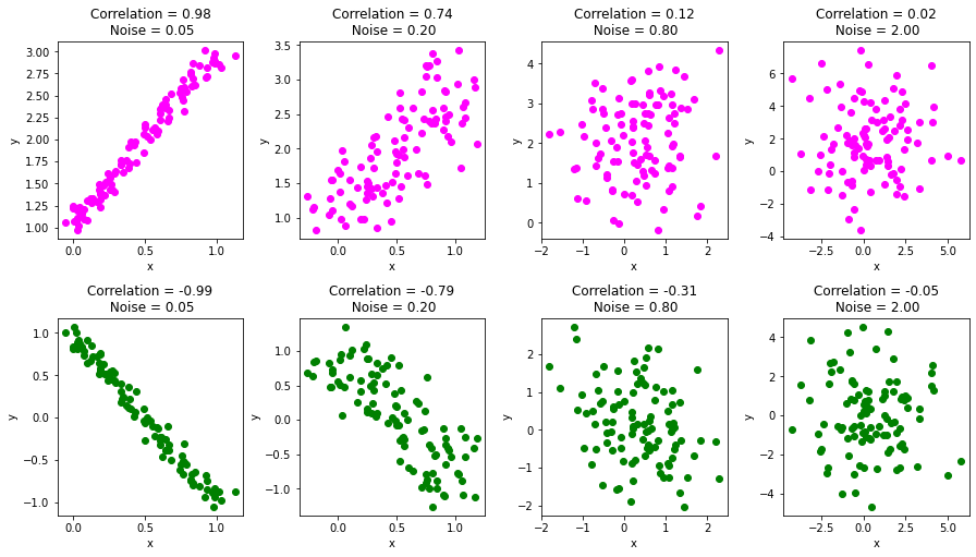
- It is bounded between -1 and +1.
  - +1: Perfect positive linear relationship.
  - -1: Perfect negative linear relationship.
  - 0: No linear relationship.
- Because it's a normalized, unit-less number, you can compare the correlation between BTC/ETH to the correlation between, say, oil and the S&P 500.

The following resource provides a great summary table and further details on these distinctions.

Covariance and Correlation: Intro, Formula, Calculation, and More

The article "Covariance and Correlation" from QuantInsti offers a clear, structured comparison.

Read the section titled "What are the differences between Covariance and Correlation?". The table in this section is an excellent summary of the four key differences regarding what they measure, their range, units, and scalability.

To solidify the visual intuition, here is how different correlation values appear in scatter plots of data.

Visualizing Correlation with Scatter Plots — This series of plots shows how the data cloud tightens into a line as the correlation coefficient approaches +1 or -1. A coefficient near zero corresponds to a formless cloud, indicating no linear relationship.

2. Under the Hood: Calculation from First Principles

Given your preference for understanding the mechanics, let's build these calculations from scratch before using any library functions. For a sample of data points (like a time series of returns), the formulas are:

Sample Covariance:

Cov (X, Y) = \frac{\sum _{i = 1}^{N} ( x _{i} - x ˉ ) ( y _{i} - y ˉ )}{N - 1}

Sample Correlation (Pearson's r):

r_{x y} = \frac{Cov ( X , Y )}{s _{x} s _{y}} = \frac{\sum _{i = 1}^{N} ( x _{i} - x ˉ ) ( y _{i} - y ˉ )}{\sum _{i = 1}^{N} ( x _{i} - x ˉ ) ^{2} \sum _{i = 1}^{N} ( y _{i} - y ˉ ) ^{2}}

where $x ˉ$ and $y ˉ$ are the sample means, and $s_{x}$ and $s_{y}$ are the sample standard deviations. The use of $N - 1$ is Bessel's correction, which you may recall from statistics.

Now, let's translate this directly into code. The following article provides a clean, step-by-step Python implementation of the Pearson correlation coefficient without using any specialized libraries like pandas or NumPy for the core logic.

Pearson Correlation Coefficient In Python | by Shivogo John - Medium

The article "Pearson Correlation Coefficient In Python" by Shivogo John provides a perfect from-scratch implementation that maps directly to the mathematical formulas.

Focus on the section "Pearson Correlation Coefficient In Python". Review the four functions provided: mean, standard_deviation, covariance, and finally pearson_correlation. Notice how each function builds upon the previous one, exactly mirroring the mathematical definitions.

This from-scratch implementation demystifies the process. It shows that .corr() in pandas isn't a black box, but an optimized implementation of these exact steps.

3. Practical Application with Python

With the theory and manual implementation understood, we can now turn to the efficient, vectorized tools provided by the pandas library. When working with financial time series, you'll almost always use these for speed and convenience.

The process involves:

Fetching price data for two or more assets into a DataFrame.
Calculating the return series for each asset. We'll continue using log returns for consistency with the previous lesson.
Using the .cov() and .corr() methods on the DataFrame of returns.

The following video demonstrates this exact workflow.

Covariance and Correlation Matrix of stock returns with Python

This clip from Algovibes, "Covariance and Correlation Matrix of stock returns with Python", shows the standard pandas workflow.

Watch from 01:23 to 07:22. Note the following steps: Calculating Returns (01:23 - 02:36): The video uses .pct_change() for simple returns. For our purposes, we'd use np.log(df / df.shift(1)) to get log returns. Covariance Matrix (02:36 - 04:23): See how .cov() is called on the returns DataFrame and how to interpret the output matrix. The diagonal elements are the variances of each asset. Correlation Matrix (04:23 - 06:17): Observe the use of .corr() and the interpretation of the resulting matrix. The diagonal is now all 1s. Visualization (06:17 - 07:22): Using a heatmap to visualize the correlation matrix is a standard and highly effective technique.

The Correlation Matrix & Heatmaps

When you have more than two assets, pandas computes a correlation matrix. This is a grid where the entry at row i and column j is the correlation between asset i and asset j.

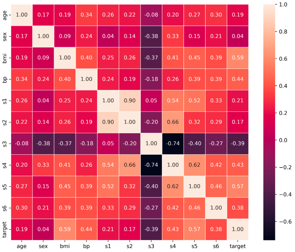
As a developer, you can think of the correlation matrix as a concise, structured representation of the pairwise relationships within a system of variables. A heatmap is simply a UI layer on top of this data structure to make it more human-readable.

4. Important Caveats

Your critical perspective on trading strategies is valuable, and it should extend to the statistical tools you use.

Correlation ≠ Causation: This is the most famous warning in statistics. If two asset prices are highly correlated, it doesn't mean one is causing the other to move. They could both be driven by a third, external factor (e.g., a change in macroeconomic policy or broad market sentiment).
Linearity: The Pearson correlation coefficient measures the strength of linear relationships only. Two variables can have a perfect non-linear relationship (e.g., $Y = X^{2}$ ) and still have a correlation of zero. Always visualize your data with a scatter plot to check for non-linear patterns.
Correlations are Unstable: The correlation between two assets is not a fixed, universal constant. It changes over time. Famously, during market crashes, the correlations between many assets tend to shoot towards +1 as investors sell everything indiscriminately. This is a critical concept for risk management. Advanced analysis often involves using rolling correlations to see how these relationships evolve.

Conclusion

In this lesson, we added two essential tools to our statistical toolkit for analyzing financial data. We learned how to measure and interpret the relationships between asset price series, moving beyond the analysis of single assets.

Key Takeaways:

Covariance measures the direction of a linear relationship but is difficult to interpret on its own because it is scale-dependent.
Correlation is a normalized measure of both the direction and strength of a linear relationship, bounded between -1 and +1.
The formulas for covariance and correlation can be implemented from scratch, but in practice, we use optimized library functions like pandas.DataFrame.corr().
A correlation matrix, often visualized with a heatmap, is the standard way to analyze pairwise relationships across multiple assets.
It's crucial to remember that correlation measures only linear relationships and does not imply causation.

Preview of the Next Lesson:

We've now seen that asset returns have properties like mean and variance, they can be modeled by distributions, and they have relationships with other assets. This complex, time-evolving behavior is best captured by modeling asset prices as a stochastic process — a process that evolves randomly through time. In the next lesson, we will formally define what a stochastic process is and explore why it's the right framework for thinking about financial markets.

Recommended resources